Article directory
- Explanation of 0 Sorting Algorithms
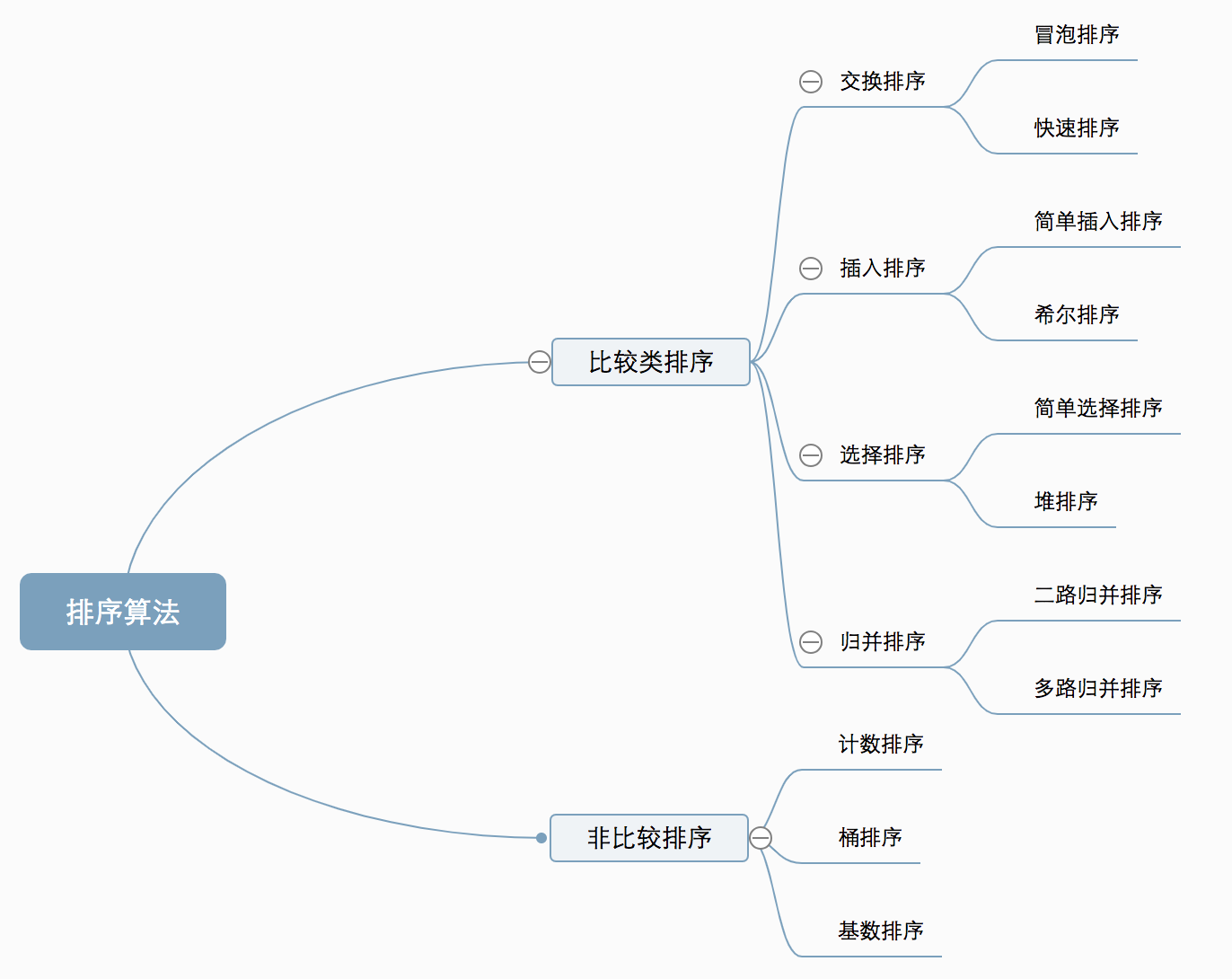
- 0.1 Internal and External Sorting
- 0.2 Comparisons and Non-Comparisons
- 0.3 On Time Complexity
- 0.4 On Stability
- 0.5 NOUN explanation:
- 1 Exchange Sort
- 1.1 When is the fastest
- 1.2 When is the slowest
- 1.3 Algorithmic Steps
- 1.4 Motion Map Demonstration
- 1.5 Java Implementation
- 2 Selection Sort
- 3 Insertion Sort
- 4 Insert Sort
- Merge Sort
- 6 Exchange Sort - Quick Sort
- 7 Selective Sort - Heap Sort
- Counting Sort
- Characteristic of 8.1 Counting Sort
- 8.2 Algorithmic Steps
- 8.3 Motion Map Demonstration
- 8.4 Java Implementation
- Bucket Sort
- 9.1 When is the fastest
- 9.2 When is the slowest
- 9.3 Algorithmic Steps
- 9.4 schematic diagram
- 9.5 Java Implementation
- Radix Sort
- 10.1 cardinal sorting vs counting sorting vs bucket sorting
- 10.2 Algorithmic Steps
- 10.3 Demonstration of LSD Cardinal Sorting Motion Map
- 10.4 Java Implementation
- Reference link
Explanation of 0 Sorting Algorithms
0.1 Internal and External Sorting
The sorting algorithm can be divided into internal sorting and external sorting. Internal sorting is the sort of data records in memory. External sorting can not accommodate all sorting records at one time because of the large size of sorted data. In the sorting process, external memory needs to be accessed.
Common internal sorting algorithms include insertion sorting, Hill sorting, selection sorting, bubble sorting, merge sorting, fast sorting, heap sorting, cardinal sorting, etc. Summarize with a picture: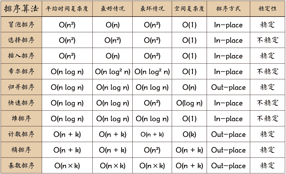

0.2 Comparisons and Non-Comparisons
Comparisons:
Common quick sort, merge sort, heap sort and bubble sort belong to comparative sort. In the final result of sorting, the order of elements depends on their comparison. Each number must be compared with other numbers in order to determine its position.
In sorting such as bubble sorting, the scale of the problem is n, and the average time complexity is O(n_) because n comparisons are needed. In sorting such as merge sorting and quick sorting, the scale of the problem is reduced to logN times by dividing and conquering, so the average time complexity is O(nlogn).
The advantage of comparative sorting is that it can be applied to data of all sizes, regardless of the distribution of data, and can be sorted. It can be said that comparative ordering is applicable to all situations where ordering is required.
Non-comparative ranking:
Counting sort, cardinal sort and bucket sort belong to non-comparative sort. Non-comparative sorting is done by determining how many elements should be sorted before each element is determined. For array arr, how many elements are calculated before arr, then the position of arr in the sorted array is determined only.
Non-comparative sorting can be solved by determining the number of existing elements before each element, and all iterations. The time complexity of the algorithm is O(n).
The time complexity of non-comparative sorting is low, but it needs space to determine the unique location because of non-comparative sorting. Therefore, there are certain requirements for data size and data distribution.
0.3 On Time Complexity
Square order (O(n^2)) sorting: all kinds of simple sorting: direct insertion, direct selection and bubble sorting.
Linear logarithmic order (O (nlog2n) sorting: fast sorting, heap sorting and merge sorting;
O(n1+) sort, is a constant between 0 and 1: Hill sort
Linear order (O (n) sorting: cardinal sorting, in addition to barrel, box sorting.
0.4 On Stability
Stable sorting algorithms: bubble sorting, insertion sorting, merge sorting and cardinal sorting.
Unstable sorting algorithm: selection sorting, fast sorting, Hill sorting, heap sorting.
0.5 NOUN explanation:
- n: Data size
- k: Number of barrels
- In-place: Constant memory, no extra memory
- Out-place: Take up extra memory
- Stability: The order of the two equivalent keys after sorting is the same as that before sorting
1 Exchange Sort
Bubble Sort is also a simple and intuitive sorting algorithm. It repeatedly visits the columns to be sorted, compares two elements at a time, and swaps them if their order is wrong. The work of visiting a sequence is repeated until no exchange is needed, that is to say, the sequence has been sorted. The algorithm's name comes from the fact that smaller elements float slowly to the top of the sequence by swapping.
1.1 When is the fastest
When the input data is in positive order (they are already in positive order, I also want you to bubble sort what is the use of ah).
1.2 When is the slowest
When the input data is in reverse order (it's not enough to write a for loop output data in reverse order, why use your bubble sort, am I idle)?
1.3 Algorithmic Steps
- Compare adjacent elements. If the first one is bigger than the second one, exchange the two.
- Do the same work for each pair of adjacent elements, from the first pair at the beginning to the last pair at the end. After this step, the final element will be the largest number.
- Repeat the above steps for all elements except the last one.
- Continue repeating the above steps for fewer and fewer elements each time until no pair of numbers need to be compared.
1.4 Motion Map Demonstration

1.5 Java Implementation
public class BubbleSort {
    public static int[] bubbleSort(int[] arr) {
        if (arr == null || arr.length == 0) {
            return arr;
        }
        for (int i = 0; i < arr.length; i++) {
            for (int j = 0; j < arr.length - i - 1; j++) {
                if (arr[j] > arr[j + 1]) {
                    int temp = arr[j];
                    arr[j] = arr[j + 1];
                    arr[j + 1] = temp;
                }
            }
        }
        return arr;
    }
}
2 Selection Sort
Direct selection sorting is a simple and intuitive sorting algorithm. No matter what data is entered, it is O(n) time complexity. So when it's used, the smaller the data size, the better. The only advantage may be that it doesn't take up extra memory space.
2.1 Algorithmic Steps
- Firstly, the smallest (large) element is found in the unordered sequence and stored at the beginning of the ordered sequence.
- Then continue to find the smallest (large) element from the remaining unordered elements, and then put it at the end of the ordered sequence.
- Repeat the second step until all elements are sorted.
2.2 Motion Map Demonstration
2.3 Java Implementation
public class SelectionSort {
    public static int[] selectionSort(int[] arr) {
        if (arr.length == 0) {
            return arr;
        }
        for (int i = 0; i < arr.length - 1; i++) {
            int minIndex = i;
            for (int j = i + 1; j < arr.length; j++) {
                if (arr[j] < arr[minIndex]) {
                    minIndex = j;
                }
            }
            if (i != minIndex) {
                int tem = arr[minIndex];
                arr[minIndex] = arr[i];
                arr[i] = tem;
            }
        }
        return arr;
    }
}
3 Insertion Sort
Although the code implementation of direct insertion sort is not as simple and crude as bubble sort and selection sort, its principle should be the easiest to understand, because anyone who has played cards should be able to understand in seconds. Insertion sort is the simplest and intuitive sort algorithm. Its working principle is to scan backward and forward in the sorted sequence to find the corresponding position and insert the unsorted data by constructing an ordered sequence.
Like bubble sort, insertion sort also has an optimization algorithm called split-and-half insertion.
3.1 Algorithmic Steps
- Consider the first element of the first sequence to be sorted as an ordered sequence, and the second element to the last element as an unordered sequence.
- Scanning the unordered sequence from beginning to end, inserting each element scanned into the appropriate position of the ordered sequence. (If the element to be inserted is equal to an element in an ordered sequence, the element to be inserted is inserted after the equivalent element.)
3.2 Motion Chart Demonstration
3.3 Java Implementation
public class InsertionSort {
    public static int[] insertionSort(int[] arr) {
        for (int i = 1; i < arr.length; i++) {
            int temp = arr[i];
            int j = i;
            while (j > 0 && temp < arr[j - 1]) {
                arr[j] = arr[j - 1];
                j--;
            }
            // Judging whether it is necessary to move or not
            if (j != i) {
                arr[j] = temp;
            }
        }
        return arr;
    }
}
4 Insert Sort
Hill sorting, also known as decreasing incremental sorting algorithm, is a more efficient improved version of insertion sorting. But Hill sorting is an unstable sorting algorithm.
Hill sort is an improved method based on the following two properties of insertion sort:
- When insertion sort is used to manipulate almost ordered data, the efficiency of insertion sort is high, and the efficiency of linear sort can be achieved.
- But insertion sort is generally inefficient, because insertion sort can only move data one bit at a time.
The basic idea of Hill sort is that the whole record sequence to be sorted is divided into several subsequences for direct insertion sort. When the records in the whole sequence are "basically ordered", then all records are directly inserted and sorted in turn.
4.1 Algorithmic Steps
- Select an incremental sequence t1, t2,... tk, where ti > tj, tk = 1;
- According to the incremental sequence number k, the sequence is sorted by K times.
- According to the corresponding incremental ti, the columns to be sorted are divided into several sub-sequences of m length, and the sub-tables are sorted directly by insertion. When the incremental factor is only 1, the whole sequence is treated as a table, and the length of the table is the length of the whole sequence.
4.2 Motion Map Demonstration
4.3 Java Implementation
public class ShellSort implements IArraySort {
    @Override
    public int[] sort(int[] sourceArray) throws Exception {
        // Copy arr without changing parameters
        int[] arr = Arrays.copyOf(sourceArray, sourceArray.length);

        int gap = 1;
        while (gap < arr.length/3) {
            gap = gap * 3 + 1;
        }

        while (gap > 0) {
            for (int i = gap; i < arr.length; i++) {
                int tmp = arr[i];
                int j = i - gap;
                while (j >= 0 && arr[j] > tmp) {
                    arr[j + gap] = arr[j];
                    j -= gap;
                }
                arr[j + gap] = tmp;
            }
            gap = (int) Math.floor(gap / 3);
        }

        return arr;
    }
}
Merge Sort
Merge sort is an effective sorting algorithm based on merge operation. This algorithm is a very typical application of Divide and Conquer.
As a typical application of divide-and-conquer algorithm, merge sorting can be realized by two methods:
- Top-down recursion (all recursive methods can be rewritten iteratively, so there is a second method);
- Bottom-up iteration;
Like selection sort, merge sort performance is not affected by input data, but it performs much better than selection sort because it is always O(nlogn) time complexity. The cost is additional memory space.
5.1 Algorithmic Steps
- The application space is the sum of two sorted sequences, which is used to store the merged sequences.
- Set two pointers, the initial position is the starting position of two sorted sequences;
- Compare the elements pointed by the two pointers, select the relatively small elements into the merge space, and move the pointer to the next position.
- Repeat step 3 until a pointer reaches the end of the sequence.
- Copy all the remaining elements of another sequence directly to the end of the merged sequence.
5.2 Motion Map Demonstration

5.3 Java Implementation
import java.util.Arrays;

public class MergeSort {
    public static int[] mergeSort(int[] arr) {
        if (arr.length < 2) {
            return arr;
        }
        int mid = arr.length / 2;
        int[] left = Arrays.copyOfRange(arr, 0, mid);
        int[] right = Arrays.copyOfRange(arr, mid, arr.length);
        int[] result = merge(mergeSort(left), mergeSort(right));
        return result;

    }

    public static int[] merge(int[] left, int[] right) {
        int len = left.length + right.length;
        int[] result = new int[len];
        int index = 0, i = 0, j = 0; // result index, left index, right index

        //        for (; index < len; index++) {
        //            if (i >= left.length) {
        //                result[index] = right[j++];
        //            } else if (j >= right.length) {
        //                result[index] = left[i++];
        //            } else if (left[i] < right[j]) {
        //                result[index] = left[i++];
        //            } else {
        //                result[index] = right[j++];
        //            }
        //        }

        //The for loop section can also be replaced by:
        while (i < left.length && j < right.length) {
            if (left[i] <= right[j]) {
                result[index++] = left[i++];
            } else {
                result[index++] = right[j++];
            }
        }
        while (i < left.length) {
            result[index++] = left[i++];
        }
        while (j < right.length) {
            result[index++] = right[j++];
        }
        return result;
    }
}
6 Exchange Sort - Quick Sort
Quick sort is a sort algorithm developed by Tony Hall. Under the average condition, n items are ranked by (nlogn) times. In the worst case, a(n2) comparison is required, but this is not common. In fact, fast sorting is usually significantly faster than other (nlogn) algorithms because its inner loop can be implemented efficiently on most architectures.
Quick sort uses Divide and conquer strategy to divide a list into two sub-lists.
Quick sorting is also a typical application of divide and conquer in sorting algorithm. Essentially, quick sorting should be regarded as a recursive divide-and-conquer method based on bubble sorting.
Quickly sorted names are simple and rude, because as soon as you hear the name, you know the meaning of its existence, that is fast and efficient! It is one of the fastest sorting algorithms for large data. Although Worst Case's time complexity is O(n_), others are excellent, and in most cases it performs better than the sorting algorithm with an average time complexity of O(n logn), but why, I don't know. Fortunately, my obsessive-compulsive disorder has been committed again. After checking N-sources, I finally found a satisfactory answer in the Competition of Algorithmic Arts and Informatics.
The worst case of quick sorting is O(n_), such as fast sorting of sequential sequences. However, its average expected time is O(nlogn), and the constant factor implied in O(nlogn) notation is very small, which is much smaller than the merge sort whose complexity is stable equal to O(nlogn). Therefore, for the vast majority of random sequence with weak order, fast sorting is always better than merging sorting.
6.1 Algorithmic Steps
- Pick out an element from a sequence called pivot.
- Reordering sequence, all elements smaller than the benchmark are placed in front of the benchmark, and all elements larger than the benchmark are placed behind the benchmark (the same number can reach either side). After the partition exits, the benchmark is in the middle of the sequence. This is called partition operation.
- Recursively, the subordinate sequence of the elements less than the reference value and the subordinate sequence of the elements larger than the reference value are sorted.
6.2 Motion Map Demonstration

6.3 Java Implementation
public class QuickSort {
    // Quick row classic "digging and filling + dividing and treating"
    public static void quickSort1(int[] arr, int start, int end) {
        if (arr.length == 0 || start >= end) {
            return;
        }
        int low = start, high = end;
        int pivot = arr[low]; // Reference value
        while (low < high) {
            while (low < high && arr[high] >= pivot) {
                high--;
            }
            if (arr[high] < pivot) {
                arr[low] = arr[high];
            }
            while (low < high && arr[low] <= pivot) {
                low++;
            }
            if (arr[low] > pivot) {
                arr[high] = arr[low];
            }
        }
        arr[low] = pivot;
        quickSort1(arr, start, low - 1);
        quickSort1(arr, low + 1, end);
    }

    // Using the Quick Sorting Algorithms in Introduction to Algorithms (3rd edition of the original book)
    // Reference is also made to the code for quick sorting recursively in Sword Finger Offer (2nd edition)
    public static void quickSort2(int[] arr, int start, int end) {
        if (arr == null || start < 0 || start > end || end >= arr.length) {
            return;
        }
        int index = partition(arr, start, end);
        if (index > start) {
            quickSort2(arr, start, index - 1);
        }
        if (index < end) {
            quickSort2(arr, index + 1, end);
        }
    }

    public static int partition(int[] arr, int start, int end) {
        int pivot = start + (int) (Math.random() * (end - start + 1));// Math.random() is a pseudo-random double value that makes the system randomly select values greater than or equal to 0.0 and less than 1.0.
        swap(arr, pivot, end);
        int smallIndex = start - 1;
        for (int i = start; i < end; i++) {
            if (arr[i] < arr[end]) {
                smallIndex++;
                if (i > smallIndex) {
                    swap(arr, i, smallIndex);
                }
            }
        }
        swap(arr, smallIndex + 1, end);
        return smallIndex + 1; // Take arr[smallIndex+1] as the dividing line, smaller in front and larger in back (range from start to end)
    }

    public static void swap(int[] arr, int i, int j) {
        int temp = arr[i];
        arr[i] = arr[j];
        arr[j] = temp;
    }
}
7 Selective Sort - Heap Sort
Heapsort is a sort algorithm designed by utilizing the data structure of heap. The heap is a nearly complete binary tree structure, and it satisfies the heap property at the same time: that is, the key value or index of the child node is always less than (or greater than) its parent node. Heap sorting can be said to be a selective sort that uses the concept of heap to sort. There are two methods:
- Big Top heap: The value of each node is greater than or equal to the value of its sub-nodes, which is used in heap sorting algorithm for ascending order.
- Small-top heap: Each node's value is less than or equal to the value of its sub-nodes, which is used for descending ranking in heap sorting algorithm.
The average time complexity of heap sorting is(nlogn).
7.1 Algorithmic Steps
- Create a heap H[0... n-1];
- Exchange the heap head (maximum) with the heap tail.
- Reduce the size of the heap by 1 and call shift_down(0) to adjust the top data of the new array to the corresponding position.
- Repeat step 2 until the heap size is 1.
7.2 Motion Chart Demonstration
7.3 Java Implementation
public class HeapSort {
    public static void heapSort(int[] arr) {
        if (arr == null || arr.length == 0) {
            return;
        }

        // Start with the last non-leaf node to create a large root heap
        for (int i = (arr.length / 2 - 1); i >= 0; i--) {
            adjustHeap(arr, i);
        }

        // Exchange and reorder the last node with the root node
        for (int i = arr.length - 1; i >= 0; i--) {
            swap(arr, 0, i);
            adjustHeap(arr, 0);
        }
    }

    // Adjust the binary tree of three nodes to make it the largest heap
    // Array and root nodes whose parameters are to be sorted
    public static void adjustHeap(int[] arr, int root) {
        int left = root * 2 + 1;
        int right = left + 1;
        int maxIndex = root;
        if (left < arr.length && arr[left] > arr[root]) {
            maxIndex = left;
        }
        if (right < arr.length && arr[right] > arr[maxIndex]) {
            maxIndex = right;
        }
        if (maxIndex != root) {
            swap(arr, root, maxIndex);
            adjustHeap(arr, maxIndex); // Change occurs after replacement, so future generations need to be readjusted.
        }
    }

    public static void swap(int[] arr, int i, int j) {
        int temp = arr[i];
        arr[i] = arr[j];
        arr[j] = temp;
    }
}
Counting Sort
The core of counting sorting is to convert the input data values into keys and store them in additional open array spaces. As a sort of linear time complexity, counting sort requires that the input data must be an integer with a certain range.
Characteristic of 8.1 Counting Sort
When the input element is an integer between N zeros and k, its running time is_ (n + k). Counting sorting is not comparative sorting, and the sorting speed is faster than any comparative sorting algorithm.
Because the length of the array C used to count depends on the range of data in the array to be sorted (equal to the difference between the maximum and minimum values of the array to be sorted plus 1), it requires a lot of time and memory for the array with a large range of data. For example, counting sort is the best algorithm for sorting numbers between 0 and 100, but it is not suitable for sorting names alphabetically. However, count sorting can be used to sort arrays with a large range of data using algorithms in cardinal sorting.
Popular understanding, for example, there are 10 people of different ages. Statistics show that 8 people are younger than A. A's age ranks ninth. With this method, we can get the position of everyone else and arrange the order. Of course, age duplication requires special processing (to ensure stability), which is why the target array is eventually backfilled and the statistics for each number subtracted by 1.
8.2 Algorithmic Steps
- Find the largest and smallest elements in the array to be sorted
- The number of occurrences of each element with a value of i in an array is counted and stored in item i of array C.
- Accumulation of all counts (starting with the first element in C, adding each item to the preceding one)
- Backfill the target array: Place each element I in item C(i) of the new array, and subtract C(i) by 1 for each element placed.
8.3 Motion Map Demonstration
8.4 Java Implementation
public class CountingSort implements IArraySort {

    @Override
    public int[] sort(int[] sourceArray) throws Exception {
        // Copy arr without changing parameters
        int[] arr = Arrays.copyOf(sourceArray, sourceArray.length);

        int maxValue = getMaxValue(arr);

        return countingSort(arr, maxValue);
    }

    private int[] countingSort(int[] arr, int maxValue) {
        int bucketLen = maxValue + 1;
        int[] bucket = new int[bucketLen];

        for (int value : arr) {
            bucket[value]++;
        }

        int sortedIndex = 0;
        for (int j = 0; j < bucketLen; j++) {
            while (bucket[j] > 0) {
                arr[sortedIndex++] = j;
                bucket[j]--;
            }
        }
        return arr;
    }

    private int getMaxValue(int[] arr) {
        int maxValue = arr[0];
        for (int value : arr) {
            if (maxValue < value) {
                maxValue = value;
            }
        }
        return maxValue;
    }
}
Bucket Sort
Bucket sorting is an upgraded version of count sorting. It makes use of the mapping relationship of functions, and the key to its efficiency lies in the determination of the mapping function. To make bucket sorting more efficient, we need to do two things:
- Increase the number of barrels as much as possible when there is enough extra space.
- The mapping function used can evenly distribute the input N data into K buckets.
At the same time, for the sorting of elements in buckets, the choice of comparative sorting algorithm is very important to the performance.
9.1 When is the fastest
When the input data can be evenly distributed to each bucket.
9.2 When is the slowest
When the input data is allocated to the same bucket.
9.3 Algorithmic Steps
- Set up a quantitative array as an empty bucket.
- Traverse the input data, and put the data one by one into the corresponding bucket;
- Sort each bucket that is not empty;
- Segmentation of sequenced data from non-empty buckets.
9.4 schematic diagram
Elements are distributed in barrels: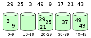
Then, the elements are sorted in each bucket: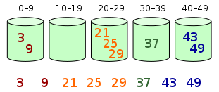
9.5 Java Implementation
public class BucketSort implements IArraySort {

    private static final InsertSort insertSort = new InsertSort();

    @Override
    public int[] sort(int[] sourceArray) throws Exception {
        // Copy arr without changing parameters
        int[] arr = Arrays.copyOf(sourceArray, sourceArray.length);

        return bucketSort(arr, 5);
    }

    private int[] bucketSort(int[] arr, int bucketSize) throws Exception {
        if (arr.length == 0) {
            return arr;
        }

        int minValue = arr[0];
        int maxValue = arr[0];
        for (int value : arr) {
            if (value < minValue) {
                minValue = value;
            } else if (value > maxValue) {
                maxValue = value;
            }
        }

        int bucketCount = (int) Math.floor((maxValue - minValue) / bucketSize) + 1;
        int[][] buckets = new int[bucketCount][0];

        // Distribution of data to buckets using mapping functions
        for (int i = 0; i < arr.length; i++) {
            int index = (int) Math.floor((arr[i] - minValue) / bucketSize);
            buckets[index] = arrAppend(buckets[index], arr[i]);
        }

        int arrIndex = 0;
        for (int[] bucket : buckets) {
            if (bucket.length <= 0) {
                continue;
            }
            // Sort each bucket, using insert sort
            bucket = insertSort.sort(bucket);
            for (int value : bucket) {
                arr[arrIndex++] = value;
            }
        }

        return arr;
    }

    /**
     * Automatically expanding and saving data
     *
     * @param arr
     * @param value
     */
    private int[] arrAppend(int[] arr, int value) {
        arr = Arrays.copyOf(arr, arr.length + 1);
        arr[arr.length - 1] = value;
        return arr;
    }

}
Radix Sort
Radix sorting is a non-comparative integer sorting algorithm. Its principle is to cut integers into different digits by digits, and then compare them by digits. Because integers can also express strings (such as names or dates) and floating-point numbers in a specific format, cardinal sorting is not limited to integers.
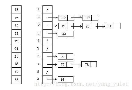
10.1 cardinal sorting vs counting sorting vs bucket sorting
There are two ways to sort cardinality:
These three sorting algorithms all use the concept of bucket, but there are obvious differences in the use of bucket.
- Cardinal sorting: Buckets are allocated according to the number of keys per digit.
- Counting sort: each bucket only stores a single key value;
- Bucket sorting: each bucket stores a range of values;
10.2 Algorithmic Steps
- Gets the maximum number in the array and the number of digits.
- arr is the original array, and each bit is taken from the lowest bit to form a radix array.
- The radix is sorted by counting (using the characteristics of counting sorting suitable for small range numbers);
10.3 Demonstration of LSD Cardinal Sorting Motion Map
10.4 Java Implementation
/**
 * Radix sorting
 * Considering negative numbers, you can also refer to https://code.i-harness.com/zh-CN/q/e98fa9.
 */
public class RadixSort implements IArraySort {

    @Override
    public int[] sort(int[] sourceArray) throws Exception {
        // Copy arr without changing parameters
        int[] arr = Arrays.copyOf(sourceArray, sourceArray.length);

        int maxDigit = getMaxDigit(arr);
        return radixSort(arr, maxDigit);
    }

    /**
     * Get the highest number of digits
     */
    private int getMaxDigit(int[] arr) {
        int maxValue = getMaxValue(arr);
        return getNumLenght(maxValue);
    }

    private int getMaxValue(int[] arr) {
        int maxValue = arr[0];
        for (int value : arr) {
            if (maxValue < value) {
                maxValue = value;
            }
        }
        return maxValue;
    }

    protected int getNumLenght(long num) {
        if (num == 0) {
            return 1;
        }
        int lenght = 0;
        for (long temp = num; temp != 0; temp /= 10) {
            lenght++;
        }
        return lenght;
    }

    private int[] radixSort(int[] arr, int maxDigit) {
        int mod = 10;
        int dev = 1;

        for (int i = 0; i < maxDigit; i++, dev *= 10, mod *= 10) {
            // Considering the negative number, we expand the number of queues by one time, where [0-9] corresponds to the negative number and [10-19] corresponds to the positive number (bucket + 10).
            int[][] counter = new int[mod * 2][0];

            for (int j = 0; j < arr.length; j++) {
                int bucket = ((arr[j] % mod) / dev) + mod;
                counter[bucket] = arrayAppend(counter[bucket], arr[j]);
            }

            int pos = 0;
            for (int[] bucket : counter) {
                for (int value : bucket) {
                    arr[pos++] = value;
                }
            }
        }

        return arr;
    }

    /**
     * Automatically expanding and saving data
     * @param arr
     * @param value
     */
    private int[] arrayAppend(int[] arr, int value) {
        arr = Arrays.copyOf(arr, arr.length + 1);
        arr[arr.length - 1] = value;
        return arr;
    }
}
Reference link
1.0 Top Ten Classical Sorting Algorithms
Top Ten Classical Sorting Algorithms (Motion Map Demonstration)