There is the concept of connected domain in mathematics, image processing and other fields. Today, I will tell you about the functions that extract the connected domain in matlab?

1, bwlabel function

bwlabel function is the simplest function to be introduced today. Its usage is as follows:

% Binary image data
BW = [ 0     1     0     0     0     0     0     0
       1     0     1     0     0     0     0     0
       0     1     0     0     0     0     1     0
       0     0     0     0     0     1     0     1
       0     0     0     0     0     0     0     0
       0     0     0     1     0     0     0     1
       0     0     1     0     0     0     0     0
       0     0     0     1     0     1     0     0 ];

% application bwlabel function
L1 = bwlabel(BW)
L2 = bwlabel(BW,4)             % Specifies that pixel connectivity is 4
L3 = bwlabel(BW,8)             % Specifies that pixel connectivity is 8

After running, it can be found that specifying pixel connectivity as 4 can not find out the connected area well. Some small partners may not be particularly familiar with pixel connectivity? Then you can see it at a glance from the figure below.

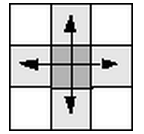
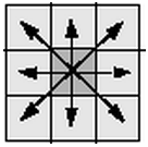
The figure above shows 4 connections and the figure below shows 8 connections. Of course, you can customize the connectivity. Don't worry first.

Generally, when using bwlabel function, just remember to use the following code instead of specifying the connectivity between pixels.

bwlabel(BW)

  2, bwlabeln function

This function is an enhanced version of the bwlabel function for n-dimensional arrays. In addition to 4-connected and 8-connected, the function also has 6-connected, 18 connected and 26 connected, and there are options for custom connectivity. The three extra connectivity are shown in the figure below:

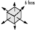
The above figure is a schematic diagram of 6 connections.

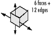
  The above figure is a schematic diagram of 18 connections.

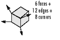
The above figure is a schematic diagram of 26 connections.

Students who have done lattice Boltzmann must be impressed.

Using this function allows you to customize connectivity, unlike bwlabel, which only allows 4 or 8. The user-defined connectivity template consists of 0 and 1. For example, the following template defines a north-south connectivity:

CONN = [ 0 1 0; 0 1 0; 0 1 0 ]

  Before using this template to judge the connectivity of the previous BW, the code is as follows:

% Define a north-south connectivity template
CONN = [ 0 1 0; 0 1 0; 0 1 0 ]

% Binary image data
BW = [ 0     1     0     0     0     0     0     0
       1     0     1     0     0     0     0     0
       0     1     0     0     0     0     1     0
       0     0     0     0     0     1     0     1
       0     0     0     1     0     0     0     1
       0     0     1     0     0     0     0     0
       0     0     0     1     0     1     0     0 ];

% Connectivity judgment
L = bwlabeln(BW,CONN)

The results are as follows:

L =

     0     2     0     0     0     0     0     0
     1     0     4     0     0     0     0     0
     0     3     0     0     0     0    10     0
     0     0     0     0     0     8     0    11
     0     0     0     0     0     0     0     0
     0     0     0     6     0     0     0    12
     0     0     5     0     0     0     0     0
     0     0     0     7     0     9     0     0

It can be found that there is no north-south connected region in the original binary image (there is no repeated equal value in L).

3, bwconncomp function

bwconncomp function is an upgraded version of bwlabeln function. It returns a structure and uses lower memory. It is recommended to use this function to judge the connectivity of binary images, because the functions of this function are basically the same as those of bwlabeln function, but it is not introduced.

But the problem is, I know where the connected area is, and how can I extract relevant information?

For example, how to find the points that belong to a common domain?

% Binary image data
BW = logical ([1     1     1     0     0     0     0     0
               1     1     1     0     1     1     0     0
               1     1     1     0     1     1     0     0
               1     1     1     0     0     0     1     0
               1     1     1     0     0     0     1     0
               1     1     1     0     0     0     1     0
               1     1     1     0     0     1     1     0
               1     1     1     0     0     0     0     0]);

% Connectivity judgment
L = bwlabel(BW,4)

% Find the point in the second connected area and return the abscissa and ordinate
[r, c] = find(L==2);
rc = [r c]

For another example, how to obtain the attributes of a connected domain?

% Binary image data
BW = [ 0     1     0     0     0     0     0     0
       1     0     1     0     0     0     0     0
       0     1     0     0     0     0     1     0
       0     0     0     0     0     1     0     1
       0     0     0     0     0     0     0     0
       0     0     0     1     0     0     0     1
       0     0     1     0     0     0     0     0
       0     0     0     1     0     1     0     0 ];

% Connectivity judgment
L = bwlabel(BW)

% Get the properties of the connected region
% s = regionprops(BW);
s = regionprops(BW,'centroid');

% Center coordinate value
centroids = cat(1, s.Centroid);

% mapping
imshow(BW)
hold on
plot(centroids(:,1),centroids(:,2), 'r*')
hold off

The effects are as follows:

It can be found that the center point of the whole image is returned, not the center point of a connected domain we want. What can we do? See the following code:

% Binary image data
BW = [ 0     1     0     0     0     0     0     0
       1     0     1     0     0     0     0     0
       0     1     0     0     0     0     1     0
       0     0     0     0     0     1     0     1
       0     0     0     0     0     0     0     0
       0     0     0     1     0     0     0     1
       0     0     1     0     0     0     0     0
       0     0     0     1     0     1     0     0 ];

% Connectivity judgment
L = bwlabel(BW)

% Get the properties of the connected region
% s = regionprops(BW);
s = regionprops(L==2,'centroid');          % Note here is L==2，Not before L

% Center coordinate value
centroids = cat(1, s.Centroid);

% mapping
imshow(BW)
hold on
plot(centroids(:,1),centroids(:,2), 'r*')
hold off

The effects are as follows:

The code perfectly returns the coordinates of the center point of the second connected domain. The regionprops function has more functions than this. Readers can check it by themselves Help documentation.