catalogue

reference material

1. Import package

2. Import data

3. View the first 5 rows of data

4. Transformation of categorical variables into dummy variables (gender)

Knowledge point - dummy variable

5. Merge data frame

6. Delete unnecessary columns

7. Count the missing value of each line

8. Visual missing value

9. View and visualize the correlation between columns

10. Discard columns with weak correlation

11. Filling of missing values

12. Delete and filter the final modeled columns

13. KNN modeling

Knowledge points - KNN

14. Forecast

reference material

• kaggle original

• Dummy variable

  • Dummy variable explanation

  • What is the dummy variable in the regression model? When do I need to set dummy variables?

1. Import package

import numpy as np
# Matrix calculation
import pandas as pd
# Data processing, such as reading data and deleting data
import seaborn as sns
# Visual template
import matplotlib.pyplot as plt
# Visual Basic Library

2. Import data

• Using PD read_ CSV () read in data

# Import data
train = pd.read_csv('E:/[Desktop]/titanic/train.csv')
test = pd.read_csv('E:/[Desktop]/titanic/test.csv')

3. View the first 5 rows of data

• Use train Head() gets the first 5 rows of data, in which you can add parameters!

print(train.head())
# Get the first 5 rows of data (default)
# You can add a parameter: train Head (6) get the first 6 lines

4. Transformation of categorical variables into dummy variables (gender)

• Original: sex -- 0 for fe male, 1 for female

• Dummy variable: it is divided into two columns, one is female and the other is male, both of which are 1 for yes and 0 for No

• Function: PD get_ Dummies(), columns passed in data frame

# Change gender column to dummy variable
train_sex = pd.get_dummies(train['Sex'])
# Turn the Sex column of the train dataset into a dummy variable
# Originally: sex 0 stands for male and 1 for female
# Dummy variable: two columns, one is male and the other is female. If it is 1, it is yes and if it is 0, it is No

Knowledge point - dummy variable

• Definition: dummy variable, also called dummy variable

• Objective: it is mainly used to deal with multi classification variables, quantify the non quantifiable multi classification variables, refine the impact of each dummy variable on the model, and improve the accuracy of the model

• Specific operation

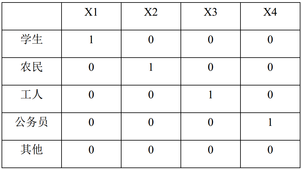
  • If the "occupational factors" column, there are five classified variables: students, farmers, workers, civil servants and others. It is transformed into 4 columns of 0 and 1 variables, so as to improve the accuracy of the model.

  • 

  Under what circumstances do you want to set dummy variables?

  1. Unordered multiclass variable

     • For example, "blood group" is divided into four types: A, B, O and AB. if it is directly assigned as 1, 2, 3 and 4, it is mathematically in order from small to large, and it is equidistant. This is inconsistent with the reality and needs to be converted into dummy variables.

  2. Ordered multiclass variable

     • For example, the severity of the disease is divided into mild, moderate and severe. If it is assigned as 1, 2, 3 (equidistant) or 1, 2, 4 (equiratio), it can reflect the hierarchical relationship, but it is inconsistent with the reality. At this time, it can be transformed into a dummy variable.

  3. Continuity variable

     • The age is very fine. Increasing the age by one year has little impact on the model and has little practical significance. We can discretize the continuous variables and divide them into 10 years old as an age group, 0 ~ 10, 11 ~ 20, 21 ~ 30, etc., represented by 1, 2, 3 and 4. At this time, it can be transformed into dummy variables, so that the impact of classification variables on the model is sufficient.

5. Merge data frame

• After the columns are converted into dummy variables, they are spliced into the data frame

• pd.concat([x, y], axis=1)

  • x and y represent the data frame to be merged

  • axis stands for splicing mode, and 1 stands for splicing by column

train = pd.concat([train, train_sex],axis=1)
# Merge the two data frames by column

The same operation not only preprocesses the training set, but also processes the test set!!!

# The same operation applies to the test set
test_sex = pd.get_dummies(test['Sex'])
test = pd.concat([test, test_sex], axis=1)

6. Delete unnecessary columns

• train.drop(['sex', 'name'], axis=1)

  • Pass in the name you want to delete

  • axis=1 means delete by column

# Discard unnecessary columns
train = train.drop(['Name', 'Sex', 'Ticket', 'Embarked'], axis=1)
# Similarly, test set
test = test.drop(['Name', 'Sex', 'Ticket','Embarked'], axis=1)

7. Count the missing value of each line

• Count the number of missing values in each column of data

print(train.isnull().sum())
print(test.isnull().sum())

8. Visual missing value

• The missing values are introduced by using the thermal diagram in the sns visualization template

• plt.show() visualizes the image

sns.heatmap(train.isnull())
# View visualization
plt.show()

9. View and visualize the correlation between columns

• train.corr() gets the correlation between the columns

• sns.heatmap() thermodynamic diagram, pass in correlation, and annot=True means to mark the correlation on the diagram!

# View the relationship between elements
print(train.corr())
​
# visualization
sns.heatmap(train.corr(), annot=True)
​
# View visualization
plt.show()

10. Discard columns with weak correlation

# Discard columns with low or weak correlation
train = train.drop(['Cabin', 'Parch', 'SibSp'], axis=1)
# Test Data
test = test.drop(['Cabin', 'Parch', 'SibSp'], axis=1)

11. Filling of missing values

# Training set
age_mean = train['Age'].mean() # Find the average of the column
train['age_mean'] = train['Age'].fillna(age_mean).apply(np.ceil) # Populate columns with missing values
​
# Test set
age_mean = test['Age'].mean()
# Gets the average value of the column
test['age_mean'] = test['Age'].fillna(age_mean).apply(np.ceil)
# . fillna() means to fill the missing values with the mean
# . apply() refers to a function applied to data, NP Ceil means that all fetches are just greater than its value -- for example, - 1.7 takes - 1
fare_mean = test['Fare'].mean()
test['Fare'] = test['Fare'].fillna(age_mean)

12. Delete and filter the final modeled columns

# Delete age column
# Training Data
train = train.drop(['Age'], axis = 1)
train.head()
# Test Data
test_new = test.drop(['PassengerId', 'Age'], axis = 1)
​
# Filter specific columns as test sets and training
X = train.loc[:, ['Pclass', 'Fare', 'female', 'male', 'age_mean']]
y = train.loc[:, ['Survived']]
# . loc [] front control row, rear control column
# Locate the corresponding row or column by name

13. KNN modeling

from sklearn.neighbors import KNeighborsClassifier
knn = KNeighborsClassifier()
# Initialize the KNN classifier, where you can set the default number and weight of neighbors of the classifier
from sklearn.model_selection import GridSearchCV
param_grid = {
    'n_neighbors': np.arange(1, 100)
}
# Set the number of neighbors traversed N
knn_cv  = GridSearchCV(knn, param_grid, cv=5)
# Get the final KNN classifier, param_grid helps to determine which N has the best classification effect from 1 to 100;
# cv indicates that the cross validation is 50% off cross validation
print(knn_cv.fit(X, y.values.ravel()))
# . values only gets the data in the data frame. Delete the column name to get an n-dimensional array
# . T ravel() returns a flat one-dimensional array
# [1,2,3], [4,5,6] becomes [1,2,3,4,5,6]
print(knn_cv.best_params_)
# Returns the size of N with the best classification effect. When the number of neighbors is, the effect is the best?
print(knn_cv.best_score_)
# Classification effect score

Knowledge points - KNN

KNN basic idea

• classification

  • To judge whether A data is A or B, it mainly depends on who its neighbors are

  • If there are more A nearby, it is considered as A; On the contrary, it is B

  • K refers to the number of neighbors, which is very important; If it is too small, it will receive individual impact; If it is too large, it will be affected by outliers in the distance; You need to try again and again

  • When calculating the distance, you can use European or Manhattan

• shortcoming

  • All distances need to be calculated, arranged from high to low; Therefore, the larger the amount of data, the lower the efficiency.

14. Forecast

• Generate forecast column

predictions = knn_cv.predict(test_new)
# Bring the test set in
​
# Submit results
submission = pd.DataFrame({
    'PassengerId': np.asarray(test.PassengerId),
    'Survived': predictions.astype(int)
})
# np.asarray() turns internal elements into arrays
# a = [1, 2]
# np.asarray(a)
# array([1, 2])
# . astype(int) converts the pandas data type to the specified data type -- int
​
# Output as csv
submission.to_csv('my_submission.csv', index=False)
# index=False indicates that the row name is not written