catalogue

1, EDA (Exploratory Data Analysis)

2, Data Preprocessing

3, Feature Engineering

4, Model Selection and Training

5, Model Ensemble

1, EDA (Exploratory Data Analysis)

• EDA: exploratory analysis of data

• Purpose:

1. Understand the meaning of each feature;
2. Know which features are useful, which can be used directly, and which can be used only after transformation, so as to prepare for future feature engineering;

• 1) Meaning and type of each feature:

  df.describe()
  df['Category'].unique()

• 2) See if missing value exists

  df.loc[df.Dates.isnull(),'Dates']

• 3) Look at the data distribution under each feature and use boxplot or hist:

  %matplotlib inline
  import matplotlib.pyplot as plt
  df.boxplot(column='Fare', by = 'Pclass')
  plt.hist(df['Fare'], bins = 10, range =(df['Fare'].min(),df['Fare'].max()))
  plt.title('Fare >distribution')
  plt.xlabel('Fare')
  plt.ylabel('Count of Passengers')

1. If the variable is categorical and you want to see distribution, you can:

   df.PdDistrict.value_counts().plot(kind='bar', figsize=(8,10))
   

2. 4) Look at the co-existence between some features, using pandas   groupby:

   temp = pd.crosstab([df.Pclass, df.Sex], df.Survived.astype(bool))
   temp.plot(kind='bar', stacked=True, color=['red','blue'], grid=False)

2, Data Preprocessing

• Objective: to process the data and prepare for model input;

1) treatment    missing   Value (missing value)

• Check whether all feature data in the dataset is missing;

1. If missing value accounts for a very small proportion of the total, fill in the average value or mode directly;
2. If the proportion of missing value is neither small nor large, its relationship with other features can be considered. If the relationship is obvious, it can be filled directly according to other features; Simple models can also be established, such as linear regression, random forest, etc.
3. If missing value accounts for a large proportion, directly treat miss value as a special case and take another value for processing;

2) handling outliers

• This is the function of EDA to find out outliers by drawing

　3)categorical feature   (category characteristics)

• Categorical   Features are often called discrete features and classification features, and the data type is usually   object   Type;

• Machine learning models can only deal with numerical data, so it is necessary to   Categorical   Data conversion to   Numeric   features.

• categorical   feature   There are two categories:

1. Ordinal   Type: this type of category has a natural order structure. If you sort the ordinal type data, it can be in ascending order or descending order. For example, in the feature of academic achievement, the specific values may include four grades: A, B, C and D, but if you sort according to the excellent results of achievement, a > b > C > D
2. Nominal type: This is a general category type and cannot sort the nominal type data. For example, the possible values of blood group characteristics are: A, B, O and AB, but you can't draw the conclusion that a > b > O > ab.

• There are different ways to convert Ordinal and Nominal data into numbers:

• Ordinal type data: Using   LabelEncoder   Coding processing;

1. For example, the grades A, B, C and D are evaluated   LabelEncoder   After processing, it will be mapped to 1, 2, 3 and 4, so that the natural size relationship between data will be preserved.

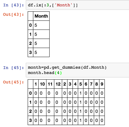
• Nominal type data: Using   OneHotEncoder   Coding processing;

1. Pandas get_dummies() method, corresponding to each virtual variable, returns a DataFrame containing a new column;
2. Use the concat() method to add these dummy columns back to the original DataFrame
3. Then drop the original columns entirely using the drop method

4) process category feature

• Generally, it is solved through dummy variable, also known as one hot encode:

1. pandas.get_dummies()
2. In sklearn   preprocessing.OneHotEncoder()

• Example:  

  Expand the month data of a column into 12 columns, and use 0 and 1 to represent the category

• 

• In addition, there are two points worth noting when dealing with category features:

1. If the feature contains a large number of dummy variable s that need to be processed, it is likely to lead to a sparse dataframe. At this time, it is best to use PCA for dimension reduction.
2. If there are tens of thousands of values for a feature, use   dummy variable   It's not realistic. You can use it at this time Count-Based Learning.

• For category features, adding TF IDF to the model has a good effect;
• "Leave one out" encoding: it can handle the problem of too many types of category features;

3, Feature Engineering

• In theory, "feature Engineering"   It belongs to data prediction.

• Feature engineering is very important. It can be said that most of the final results are determined by feature engineering, and the rest should be involved   Ensemble (integrated learning)   decision.

• The quality of characteristic engineering is mainly determined by   domain knowledge   Yes, but most people may not have this knowledge, so they can only generate new features based on the original features as much as possible, and then let the model select the important features. Here it comes to   feature selection;

• feature selection   Methods: backward and forward selection   Wait a lot. I personally prefer to use   random forest   of   feature importance， here This method is introduced in some papers.

4, Model Selection and Training

1) Model Selection

• The most commonly used model is   Ensemble Model, such as   Random Forest,Gradient Boosting.

• For the project on Kaggle, a simple model can be used at the beginning. On the one hand, it can be used as the bottom line threshold, on the other hand, it can also be used as the assembly model at the end. xgboost

2) Model Training

• The training model is mainly parameter adjustment. Each model has its own key parameters in sklearn

1. GridSearchCV   (grid search) set several parameter combinations to be compared;

2. use   cross validation   Select the best parameter combination.

• General usage:

  from sklearn.grid_search import GridSearchCV
  from pprint import pprint
  clf=RandomForestClassifier(random_state=seed)
  parameters = {'n_estimators': [300, 500], 'max_features':[4,5,'auto']}
  grid_search = GridSearchCV(estimator=clf,param_grid=parameters, cv=10, scoring='accuracy')
  print("parameters:")
  pprint(parameters)
  grid_search.fit(train_x,train_y)
  print("Best score: %0.3f" % grid_search.best_score_)
  print("Best parameters set:")
  best_parameters=grid_search.best_estimator_.get_params()
  for param_name in sorted(parameters.keys()):
  print("\t%s: %r" % (param_name, best_parameters[param_name]))

5, Model Ensemble

• Model Ensemble   Methods: Pasting, bagging, boosting and Stacking; among   Bagging   and   Boosting   It's all   Bootstraping   Application of. Bootstraping   The concept of sampling is to take back samples every time, sampling K samples, a total of N times.

• Bagging: randomly select K samples from the population samples to train the model each time, repeat N times to obtain N models, then merge the results of each model, combine the voting methods of classification problems, and take the average value for regression, e.g.Random Forest.

• Boosting: at first, give each sample the same weight, and then iterate the training. Each time, increase the weight of the training failed sample. Finally, multiple models are combined by weighted average, e.g. GBDT.

• Comparison between Bagging and boosting: after in-depth understanding of Bagging and boosting, it is found that Bagging actually uses the same model to train randomly sampled data. This result is the difference between various models   Bias is almost the same, and variance is almost the same. Through the average, make   variance   Reduce (as can be seen from the formula for calculating the average variance), so as to improve   ensemble model   Performance. and   Boosting is actually a greedy algorithm that keeps reducing bias.

• Stacking: train one model to combine other models.

1. Firstly, several different models are trained;
2. Then train a model with the output of each model trained before as the input to get a final output.

• stacking is much like a neural network. It constructs the middle layer through the output of many models, and finally uses logical regression to train the middle layer to get the final result.
• Example:

  def single_model_stacking(clf):
       skf = list(StratifiedKFold(y, 10))
       dataset_blend_train = np.zeros((Xtrain.shape[0],len(set(y.tolist()))))
      dataset_blend_test = np.zeros((Xtest.shape[0],len(set(y.tolist()))))
      dataset_blend_test_list=[]
      loglossList=[]
      for i, (train, test) in enumerate(skf):
      dataset_blend_test_j = []
      X_train = Xtrain[train]
      y_train =dummy_y[train]
      X_val = Xtrain[test]
      y_val = dummy_y[test]
      if clf=='NN_fit':
          fold_pred,pred=NN_fit(X_train, y_train,X_val,y_val)
      if clf=='xgb_fit':
               fold_pred,pred=xgb_fit(X_train, y_train,X_val,y_val)
      if clf=='lr_fit':
          fold_pred,pred=lr_fit(X_train, y_train,X_val,y_val) 
      print('Fold %d, logloss:%f '%(i,log_loss(y_val,fold_pred))) 
  
      dataset_blend_train[test, :] = fold_pred                 
      dataset_blend_test_list.append( pred )         
      loglossList.append(log_loss(y_val,fold_pred))     
      dataset_blend_test = np.mean(dataset_blend_test_list,axis=0)    
      print('average log loss is :',np.mean(log_loss(y_val,fold_pred)))
      print ("Blending.")
  
      clf = LogisticRegression(multi_class='multinomial',solver='lbfgs')     
      clf.fit(dataset_blend_train, np.argmax(dummy_y,axis=1))
      pred = clf.predict_proba(dataset_blend_test)
  
      return pred