preface
In order to record my learning process, I have roughly sorted out the analysis process. The tool is to use Jupiter notebook, which I prefer, and then export it into md format and send it to csdn to share with you;
This is only a simple analysis process, so it is relatively simple. If there is something wrong, I hope you can include it more. You are also welcome to exchange opinions.
Table of Contents
import numpy as np
import pandas as pd

import matplotlib.pyplot as plt
import matplotlib
matplotlib.rcParams['font.family'] = 'STSong'
import seaborn as sns
from sklearn.ensemble import RandomForestClassifier
from sklearn.preprocessing import OneHotEncoder, LabelEncoder, StandardScaler


import warnings
warnings.filterwarnings('ignore')
data fetch
df_train = pd.read_csv('../titanic_dir/titanic_data/train.csv')
df_test = pd.read_csv('../titanic_dir/titanic_data/test.csv')
df_all = pd.concat([df_train, df_test])
df_all.reset_index(drop=True,inplace=True)

print('df_all'+'*'*20)
print(df_all.columns)

print('df_train'+'*'*20)
print(df_train.columns)

print('df_test'+'*'*20)
print(df_test.columns)
df_all********************
Index(['PassengerId', 'Survived', 'Pclass', 'Name', 'Sex', 'Age', 'SibSp',
       'Parch', 'Ticket', 'Fare', 'Cabin', 'Embarked'],
      dtype='object')
df_train********************
Index(['PassengerId', 'Survived', 'Pclass', 'Name', 'Sex', 'Age', 'SibSp',
       'Parch', 'Ticket', 'Fare', 'Cabin', 'Embarked'],
      dtype='object')
df_test********************
Index(['PassengerId', 'Pclass', 'Name', 'Sex', 'Age', 'SibSp', 'Parch',
       'Ticket', 'Fare', 'Cabin', 'Embarked'],
      dtype='object')
df_all
| PassengerId | Survived | Pclass | Name | Sex | Age | SibSp | Parch | Ticket | Fare | Cabin | Embarked | |
|---|---|---|---|---|---|---|---|---|---|---|---|---|
| 0 | 1 | 0.0 | 3 | Braund, Mr. Owen Harris | male | 22.0 | 1 | 0 | A/5 21171 | 7.2500 | NaN | S |
| 1 | 2 | 1.0 | 1 | Cumings, Mrs. John Bradley (Florence Briggs Th... | female | 38.0 | 1 | 0 | PC 17599 | 71.2833 | C85 | C |
| 2 | 3 | 1.0 | 3 | Heikkinen, Miss. Laina | female | 26.0 | 0 | 0 | STON/O2. 3101282 | 7.9250 | NaN | S |
| 3 | 4 | 1.0 | 1 | Futrelle, Mrs. Jacques Heath (Lily May Peel) | female | 35.0 | 1 | 0 | 113803 | 53.1000 | C123 | S |
| 4 | 5 | 0.0 | 3 | Allen, Mr. William Henry | male | 35.0 | 0 | 0 | 373450 | 8.0500 | NaN | S |
| ... | ... | ... | ... | ... | ... | ... | ... | ... | ... | ... | ... | ... |
| 1304 | 1305 | NaN | 3 | Spector, Mr. Woolf | male | NaN | 0 | 0 | A.5. 3236 | 8.0500 | NaN | S |
| 1305 | 1306 | NaN | 1 | Oliva y Ocana, Dona. Fermina | female | 39.0 | 0 | 0 | PC 17758 | 108.9000 | C105 | C |
| 1306 | 1307 | NaN | 3 | Saether, Mr. Simon Sivertsen | male | 38.5 | 0 | 0 | SOTON/O.Q. 3101262 | 7.2500 | NaN | S |
| 1307 | 1308 | NaN | 3 | Ware, Mr. Frederick | male | NaN | 0 | 0 | 359309 | 8.0500 | NaN | S |
| 1308 | 1309 | NaN | 3 | Peter, Master. Michael J | male | NaN | 1 | 1 | 2668 | 22.3583 | NaN | C |
1309 rows × 12 columns
df_all.info()
<class 'pandas.core.frame.DataFrame'>
RangeIndex: 1309 entries, 0 to 1308
Data columns (total 12 columns):
 #   Column       Non-Null Count  Dtype
---  ------       --------------  -----
 0   PassengerId  1309 non-null   int64
 1   Survived     891 non-null    float64
 2   Pclass       1309 non-null   int64
 3   Name         1309 non-null   object
 4   Sex          1309 non-null   object
 5   Age          1046 non-null   float64
 6   SibSp        1309 non-null   int64
 7   Parch        1309 non-null   int64
 8   Ticket       1309 non-null   object
 9   Fare         1308 non-null   float64
 10  Cabin        295 non-null    object
 11  Embarked     1307 non-null   object
dtypes: float64(3), int64(4), object(5)
memory usage: 122.8+ KB
The missing rate of Age and Cabin data is large;
Embarked, the deletion rate of far is very small
feature correlation
Pearson correlation formula

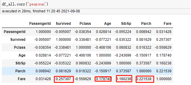
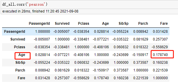
df_all.corr('pearson')
| PassengerId | Survived | Pclass | Age | SibSp | Parch | Fare | |
|---|---|---|---|---|---|---|---|
| PassengerId | 1.000000 | -0.005007 | -0.038354 | 0.028814 | -0.055224 | 0.008942 | 0.031428 |
| Survived | -0.005007 | 1.000000 | -0.338481 | -0.077221 | -0.035322 | 0.081629 | 0.257307 |
| Pclass | -0.038354 | -0.338481 | 1.000000 | -0.408106 | 0.060832 | 0.018322 | -0.558629 |
| Age | 0.028814 | -0.077221 | -0.408106 | 1.000000 | -0.243699 | -0.150917 | 0.178740 |
| SibSp | -0.055224 | -0.035322 | 0.060832 | -0.243699 | 1.000000 | 0.373587 | 0.160238 |
| Parch | 0.008942 | 0.081629 | 0.018322 | -0.150917 | 0.373587 | 1.000000 | 0.221539 |
| Fare | 0.031428 | 0.257307 | -0.558629 | 0.178740 | 0.160238 | 0.221539 | 1.000000 |
Data filling
df_all
| PassengerId | Survived | Pclass | Name | Sex | Age | SibSp | Parch | Ticket | Fare | Cabin | Embarked | |
|---|---|---|---|---|---|---|---|---|---|---|---|---|
| 0 | 1 | 0.0 | 3 | Braund, Mr. Owen Harris | male | 22.0 | 1 | 0 | A/5 21171 | 7.2500 | NaN | S |
| 1 | 2 | 1.0 | 1 | Cumings, Mrs. John Bradley (Florence Briggs Th... | female | 38.0 | 1 | 0 | PC 17599 | 71.2833 | C85 | C |
| 2 | 3 | 1.0 | 3 | Heikkinen, Miss. Laina | female | 26.0 | 0 | 0 | STON/O2. 3101282 | 7.9250 | NaN | S |
| 3 | 4 | 1.0 | 1 | Futrelle, Mrs. Jacques Heath (Lily May Peel) | female | 35.0 | 1 | 0 | 113803 | 53.1000 | C123 | S |
| 4 | 5 | 0.0 | 3 | Allen, Mr. William Henry | male | 35.0 | 0 | 0 | 373450 | 8.0500 | NaN | S |
| ... | ... | ... | ... | ... | ... | ... | ... | ... | ... | ... | ... | ... |
| 1304 | 1305 | NaN | 3 | Spector, Mr. Woolf | male | NaN | 0 | 0 | A.5. 3236 | 8.0500 | NaN | S |
| 1305 | 1306 | NaN | 1 | Oliva y Ocana, Dona. Fermina | female | 39.0 | 0 | 0 | PC 17758 | 108.9000 | C105 | C |
| 1306 | 1307 | NaN | 3 | Saether, Mr. Simon Sivertsen | male | 38.5 | 0 | 0 | SOTON/O.Q. 3101262 | 7.2500 | NaN | S |
| 1307 | 1308 | NaN | 3 | Ware, Mr. Frederick | male | NaN | 0 | 0 | 359309 | 8.0500 | NaN | S |
| 1308 | 1309 | NaN | 3 | Peter, Master. Michael J | male | NaN | 1 | 1 | 2668 | 22.3583 | NaN | C |
1309 rows × 12 columns
Fare
df_all[df_all['Fare'].isnull()]
| PassengerId | Survived | Pclass | Name | Sex | Age | SibSp | Parch | Ticket | Fare | Cabin | Embarked | |
|---|---|---|---|---|---|---|---|---|---|---|---|---|
| 1043 | 1044 | NaN | 3 | Storey, Mr. Thomas | male | 60.5 | 0 | 0 | 3701 | NaN | NaN | S |
There is only one missing data in Fare, and it comes from the test verification data, so the observed is empty. The correlation between Age, sibsp and parch and Fare is greater than 0.1, and these three values in this line of data are not empty, but the Age here is a continuous value, which is difficult to group. Considering that there is only one missing data, Age is discarded because gender is generally considered, So finally, Sex is also added, so the median after grouping the three attributes SibSp,Parch and Sex - groupby is filled here
df_all.groupby(['Parch', 'SibSp','Sex'])['Fare'].median()
# df_all.groupby(['Parch', 'Age', 'SibSp','Sex'])['Fare'].median().to_clipboard()
Parch  SibSp  Sex
0      0      female     10.50000
              male        8.05000
       1      female     26.00000
              male       26.00000
       2      female     23.25000
              male       23.25000
       3      female     18.42500
              male       18.00000
1      0      female     39.40000
              male       33.00000
       1      female     26.00000
              male       23.00000
       2      female     23.00000
              male       25.25000
       3      female     25.46670
              male       21.55000
       4      male       34.40625
2      0      female     22.35830
              male       30.75000
       1      female     41.57920
              male       41.57920
       2      female    148.37500
              male      148.37500
       3      female    263.00000
              male       27.90000
       4      female     31.27500
              male       31.38750
       5      female     46.90000
              male       46.90000
       8      female     69.55000
              male       69.55000
3      0      female     29.12915
       1      female     34.37500
              male      148.37500
       2      female     18.75000
4      0      female     23.27085
       1      female    145.45000
              male      145.45000
5      0      female     34.40625
       1      female     31.33125
              male       31.33125
6      1      female     46.90000
              male       46.90000
9      1      female     69.55000
              male       69.55000
Name: Fare, dtype: float64
Parch: 0, sibsp: 0, sex: male: 8.05000
df_all['Fare'] = df_all['Fare'].fillna(8.05000)
df_all[df_all['Fare'].isnull()]
| PassengerId | Survived | Pclass | Name | Sex | Age | SibSp | Parch | Ticket | Fare | Cabin | Embarked |
|---|
Age
263 rows missing Age
According to the Pearson correlation table, there are only Fare and Age related in all digital fields
Age, embarked and cabin can be considered for subsequent optimization
df_all['Age'].isnull().value_counts()
False    1046
True      263
Name: Age, dtype: int64
Observe the Age field and Fare
Take a look at the data distribution of Fare
plt.figure(figsize=(15,10))
plt.hist(df_all['Fare'])
plt.show()
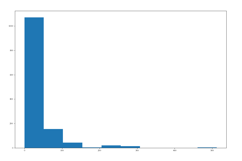
Most fare s are in the range of 0-50
# Isometric segmentation
df_all['Fare_cut'] = pd.qcut(df_all['Fare'],10)
plt.figure(figsize=(15,10))
df_all['Fare_cut'].value_counts().plot(kind='bar',rot=30)
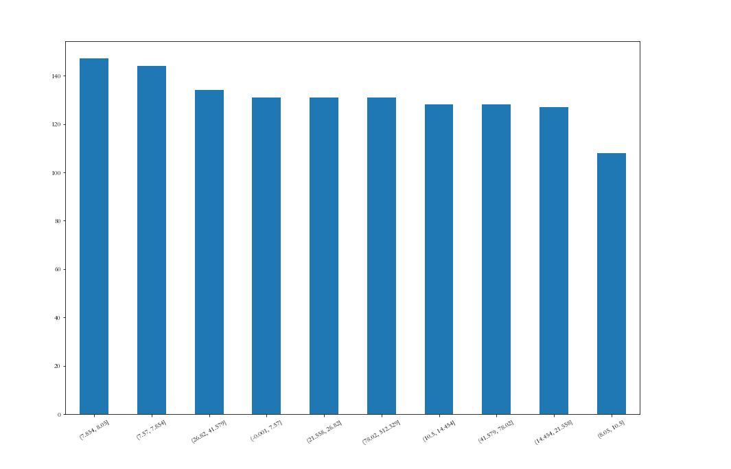
<AxesSubplot:>
Far is equally divided into 10 intervals
df_all.groupby(['Fare_cut','Sex']).agg({'Age':'median'})
| Age | ||
|---|---|---|
| Fare_cut | Sex | |
| (-0.001, 7.57] | female | 20.25 |
| male | 25.00 | |
| (7.57, 7.854] | female | 22.00 |
| male | 25.00 | |
| (7.854, 8.05] | female | 24.00 |
| male | 28.00 | |
| (8.05, 10.5] | female | 22.50 |
| male | 24.50 | |
| (10.5, 14.454] | female | 27.00 |
| male | 30.00 | |
| (14.454, 21.558] | female | 24.00 |
| male | 26.00 | |
| (21.558, 26.82] | female | 29.00 |
| male | 36.00 | |
| (26.82, 41.579] | female | 24.00 |
| male | 29.00 | |
| (41.579, 78.02] | female | 35.00 |
| male | 32.00 | |
| (78.02, 512.329] | female | 35.00 |
| male | 37.00 |
Group by. Transform after grouping, fill in with the median Age in the group (transform is really easy to use!!! Readers are recommended to learn more about Baidu)
df_all['Age'] = df_all.groupby(['Fare_cut','Sex'])['Age'].transform(lambda x:x.fillna(x.median()))
df_all['Age'].isnull().value_counts()
False    1309
Name: Age, dtype: int64
The difference between apply and transform in groupby
list(df_all.groupby(['Fare_cut','Sex']))
[((Interval(-0.001, 7.57, closed='right'), 'female'),
        PassengerId  Survived  Pclass  \
  19             20       1.0       3
  235           236       0.0       3
  367           368       1.0       3
  376           377       1.0       3
  649           650       1.0       3
  654           655       0.0       3
  780           781       1.0       3
  786           787       1.0       3
  875           876       1.0       3
  892           893       NaN       3
  899           900       NaN       3
  910           911       NaN       3
  1004         1005       NaN       3
  1182         1183       NaN       3
  1238         1239       NaN       3
The data operated by apply in group by can be series or dataframe
The data operated by the transform in groupby can only be series
The following apply groups directly
df_all.groupby(['Fare_cut','Sex'])['Age','Fare'].apply(lambda x:x.count())
| Age | Fare | ||
|---|---|---|---|
| Fare_cut | Sex | ||
| (-0.001, 7.57] | female | 15 | 15 |
| male | 116 | 116 | |
| (7.57, 7.854] | female | 50 | 50 |
| male | 94 | 94 | |
| (7.854, 8.05] | female | 22 | 22 |
| male | 125 | 125 | |
| (8.05, 10.5] | female | 30 | 30 |
| male | 78 | 78 | |
| (10.5, 14.454] | female | 49 | 49 |
| male | 79 | 79 | |
| (14.454, 21.558] | female | 61 | 61 |
| male | 66 | 66 | |
| (21.558, 26.82] | female | 52 | 52 |
| male | 79 | 79 | |
| (26.82, 41.579] | female | 52 | 52 |
| male | 82 | 82 | |
| (41.579, 78.02] | female | 53 | 53 |
| male | 75 | 75 | |
| (78.02, 512.329] | female | 82 | 82 |
| male | 49 | 49 |
In the following apply, the X passed in is a dataframe. If you need to operate on a single column, you can use x.iloc[:,0]
df_all.groupby(['Fare_cut','Sex'])['Age','Fare'].apply(lambda x:x.iloc[:,0].count()+x.iloc[:,1].count())
# df_all.groupby(['Fare_cut','Sex'])['Age','Fare'].apply(lambda x:print(type(x)))
Fare_cut          Sex
(-0.001, 7.57]    female     30
                  male      232
(7.57, 7.854]     female    100
                  male      188
(7.854, 8.05]     female     44
                  male      250
(8.05, 10.5]      female     60
                  male      156
(10.5, 14.454]    female     98
                  male      158
(14.454, 21.558]  female    122
                  male      132
(21.558, 26.82]   female    104
                  male      158
(26.82, 41.579]   female    104
                  male      164
(41.579, 78.02]   female    106
                  male      150
(78.02, 512.329]  female    164
                  male       98
dtype: int64
Embarked
df_all[df_all['Embarked'].isnull()]
| PassengerId | Survived | Pclass | Name | Sex | Age | SibSp | Parch | Ticket | Fare | Cabin | Embarked | Fare_cut | |
|---|---|---|---|---|---|---|---|---|---|---|---|---|---|
| 61 | 62 | 1.0 | 1 | Icard, Miss. Amelie | female | 38.0 | 0 | 0 | 113572 | 80.0 | B28 | NaN | (78.02, 512.329] |
| 829 | 830 | 1.0 | 1 | Stone, Mrs. George Nelson (Martha Evelyn) | female | 62.0 | 0 | 0 | 113572 | 80.0 | B28 | NaN | (78.02, 512.329] |
df_all.groupby(['Fare_cut','Sex','Embarked'])['Embarked'].count()
Fare_cut          Sex     Embarked
(-0.001, 7.57]    female  C             7
                          Q             3
                          S             5
                  male    C            42
                          Q             4
                          S            70
(7.57, 7.854]     female  C             0
                          Q            34
                          S            16
                  male    C             0
                          Q            38
                          S            56
(7.854, 8.05]     female  C             0
                          Q             8
                          S            14
                  male    C             6
                          Q             2
                          S           117
(8.05, 10.5]      female  C             1
                          Q             1
                          S            28
                  male    C             3
                          Q             2
                          S            73
(10.5, 14.454]    female  C            12
                          Q             2
                          S            35
                  male    C            11
                          Q             4
                          S            64
(14.454, 21.558]  female  C            13
                          Q             6
                          S            42
                  male    C            15
                          Q             4
                          S            47
(21.558, 26.82]   female  C             3
                          Q             3
                          S            46
                  male    C             8
                          Q             3
                          S            68
(26.82, 41.579]   female  C            15
                          Q             1
                          S            36
                  male    C            27
                          Q             5
                          S            50
(41.579, 78.02]   female  C            20
                          Q             0
                          S            33
                  male    C            17
                          Q             0
                          S            58
(78.02, 512.329]  female  C            42
                          Q             2
                          S            36
                  male    C            28
                          Q             1
                          S            20
Name: Embarked, dtype: int64

The missing two lines are both women and the cost is 80 yuan
Here, use the corresponding:
The ticket price is between (78.051, 512.329]
Among women, the largest number is C
# Filling the missing values in Embarked with S
df_all['Embarked'] = df_all['Embarked'].fillna('C')
df_all[df_all['Embarked'].isnull()]
| PassengerId | Survived | Pclass | Name | Sex | Age | SibSp | Parch | Ticket | Fare | Cabin | Embarked | Fare_cut |
|---|
Cabin
df_all['Cabin'].isnull().value_counts()
True     1014
False     295
Name: Cabin, dtype: int64
The bin attribute has many missing values. Here, M is used to fill in the missing values temporarily, and the others are replaced by the initial letter
df_all['Cabin'] = df_all['Cabin'].fillna('M')
# The missing value is replaced by M
df_all['Cabin_new'] = df_all['Cabin'].apply(lambda x:x[0])
df_all['Cabin_new'].value_counts()
M    1014
C      94
B      65
D      46
E      41
A      22
F      21
G       5
T       1
Name: Cabin_new, dtype: int64
End of missing value supplement
df_all.info()
<class 'pandas.core.frame.DataFrame'>
RangeIndex: 1309 entries, 0 to 1308
Data columns (total 14 columns):
 #   Column       Non-Null Count  Dtype
---  ------       --------------  -----
 0   PassengerId  1309 non-null   int64
 1   Survived     891 non-null    float64
 2   Pclass       1309 non-null   int64
 3   Name         1309 non-null   object
 4   Sex          1309 non-null   object
 5   Age          1309 non-null   float64
 6   SibSp        1309 non-null   int64
 7   Parch        1309 non-null   int64
 8   Ticket       1309 non-null   object
 9   Fare         1309 non-null   float64
 10  Cabin        1309 non-null   object
 11  Embarked     1309 non-null   object
 12  Fare_cut     1309 non-null   category
 13  Cabin_new    1309 non-null   object
dtypes: category(1), float64(3), int64(4), object(6)
memory usage: 135.1+ KB
df_all_copy = df_all.copy()
# Data backup
Rescued analysis
df_all
| PassengerId | Survived | Pclass | Name | Sex | Age | SibSp | Parch | Ticket | Fare | Cabin | Embarked | Fare_cut | Cabin_new | |
|---|---|---|---|---|---|---|---|---|---|---|---|---|---|---|
| 0 | 1 | 0.0 | 3 | Braund, Mr. Owen Harris | male | 22.0 | 1 | 0 | A/5 21171 | 7.2500 | M | S | (-0.001, 7.57] | M |
| 1 | 2 | 1.0 | 1 | Cumings, Mrs. John Bradley (Florence Briggs Th... | female | 38.0 | 1 | 0 | PC 17599 | 71.2833 | C85 | C | (41.579, 78.02] | C |
| 2 | 3 | 1.0 | 3 | Heikkinen, Miss. Laina | female | 26.0 | 0 | 0 | STON/O2. 3101282 | 7.9250 | M | S | (7.854, 8.05] | M |
| 3 | 4 | 1.0 | 1 | Futrelle, Mrs. Jacques Heath (Lily May Peel) | female | 35.0 | 1 | 0 | 113803 | 53.1000 | C123 | S | (41.579, 78.02] | C |
| 4 | 5 | 0.0 | 3 | Allen, Mr. William Henry | male | 35.0 | 0 | 0 | 373450 | 8.0500 | M | S | (7.854, 8.05] | M |
| ... | ... | ... | ... | ... | ... | ... | ... | ... | ... | ... | ... | ... | ... | ... |
| 1304 | 1305 | NaN | 3 | Spector, Mr. Woolf | male | 28.0 | 0 | 0 | A.5. 3236 | 8.0500 | M | S | (7.854, 8.05] | M |
| 1305 | 1306 | NaN | 1 | Oliva y Ocana, Dona. Fermina | female | 39.0 | 0 | 0 | PC 17758 | 108.9000 | C105 | C | (78.02, 512.329] | C |
| 1306 | 1307 | NaN | 3 | Saether, Mr. Simon Sivertsen | male | 38.5 | 0 | 0 | SOTON/O.Q. 3101262 | 7.2500 | M | S | (-0.001, 7.57] | M |
| 1307 | 1308 | NaN | 3 | Ware, Mr. Frederick | male | 28.0 | 0 | 0 | 359309 | 8.0500 | M | S | (7.854, 8.05] | M |
| 1308 | 1309 | NaN | 3 | Peter, Master. Michael J | male | 36.0 | 1 | 1 | 2668 | 22.3583 | M | C | (21.558, 26.82] | M |
1309 rows × 14 columns
survived_sum = df_train['Survived'].value_counts().sum()
df_train['Survived'].value_counts()/ survived_sum
0    0.616162
1    0.383838
Name: Survived, dtype: float64
(df_train['Survived'].value_counts()/ survived_sum).plot(kind='bar')
<AxesSubplot:>
The probability of being rescued in training concentration is about 38%
Feature Engineering
Fare
del df_all['Fare_cut']
df_all[:2]
| PassengerId | Survived | Pclass | Name | Sex | Age | SibSp | Parch | Ticket | Fare | Cabin | Embarked | Cabin_new | |
|---|---|---|---|---|---|---|---|---|---|---|---|---|---|
| 0 | 1 | 0.0 | 3 | Braund, Mr. Owen Harris | male | 22.0 | 1 | 0 | A/5 21171 | 7.2500 | M | S | M |
| 1 | 2 | 1.0 | 1 | Cumings, Mrs. John Bradley (Florence Briggs Th... | female | 38.0 | 1 | 0 | PC 17599 | 71.2833 | C85 | C | C |
When filling in the missing value for the Age attribute, the far field is divided into 10 intervals, and a new attribute far_cut is created, which is deleted here
Cabin
df_all['Cabin'] = df_all['Cabin_new']
del df_all['Cabin_new']
df_all[:2]
| PassengerId | Survived | Pclass | Name | Sex | Age | SibSp | Parch | Ticket | Fare | Cabin | Embarked | |
|---|---|---|---|---|---|---|---|---|---|---|---|---|
| 0 | 1 | 0.0 | 3 | Braund, Mr. Owen Harris | male | 22.0 | 1 | 0 | A/5 21171 | 7.2500 | M | S |
| 1 | 2 | 1.0 | 1 | Cumings, Mrs. John Bradley (Florence Briggs Th... | female | 38.0 | 1 | 0 | PC 17599 | 71.2833 | C | C |
Replace bin with the value of the newly built attribute bin_new
Age
Not yet
New feature --- family_size
df_all['Family_Size'] = df_all['SibSp'] + df_all['Parch'] + 1
Add 1 to SibSp and Parch to obtain the value of Family_Size
df_all[:2]
| PassengerId | Survived | Pclass | Name | Sex | Age | SibSp | Parch | Ticket | Fare | Cabin | Embarked | Family_Size | |
|---|---|---|---|---|---|---|---|---|---|---|---|---|---|
| 0 | 1 | 0.0 | 3 | Braund, Mr. Owen Harris | male | 22.0 | 1 | 0 | A/5 21171 | 7.2500 | M | S | 2 |
| 1 | 2 | 1.0 | 1 | Cumings, Mrs. John Bradley (Florence Briggs Th... | female | 38.0 | 1 | 0 | PC 17599 | 71.2833 | C | C | 2 |
New feature --- title
df_all['Name'].str.split(', ', expand=True)
| 0 | 1 | |
|---|---|---|
| 0 | Braund | Mr. Owen Harris |
| 1 | Cumings | Mrs. John Bradley (Florence Briggs Thayer) |
| 2 | Heikkinen | Miss. Laina |
| 3 | Futrelle | Mrs. Jacques Heath (Lily May Peel) |
| 4 | Allen | Mr. William Henry |
| ... | ... | ... |
| 1304 | Spector | Mr. Woolf |
| 1305 | Oliva y Ocana | Dona. Fermina |
| 1306 | Saether | Mr. Simon Sivertsen |
| 1307 | Ware | Mr. Frederick |
| 1308 | Peter | Master. Michael J |
1309 rows × 2 columns
Extract the prefix in the Name field
df_all['Title'] = df_all['Name'].str.split(', ', expand=True)[1].str.split('.', expand=True)[0]
df_all['Title'].value_counts()
Mr              757
Miss            260
Mrs             197
Master           61
Dr                8
Rev               8
Col               4
Major             2
Mlle              2
Ms                2
Lady              1
Capt              1
Jonkheer          1
Mme               1
Dona              1
Sir               1
the Countess      1
Don               1
Name: Title, dtype: int64
plt.subplots(figsize=(20, 10))
sns.barplot(x=df_all['Title'].value_counts().index, y=df_all['Title'].value_counts().values)
plt.title('Number of prefixes')
plt.show()
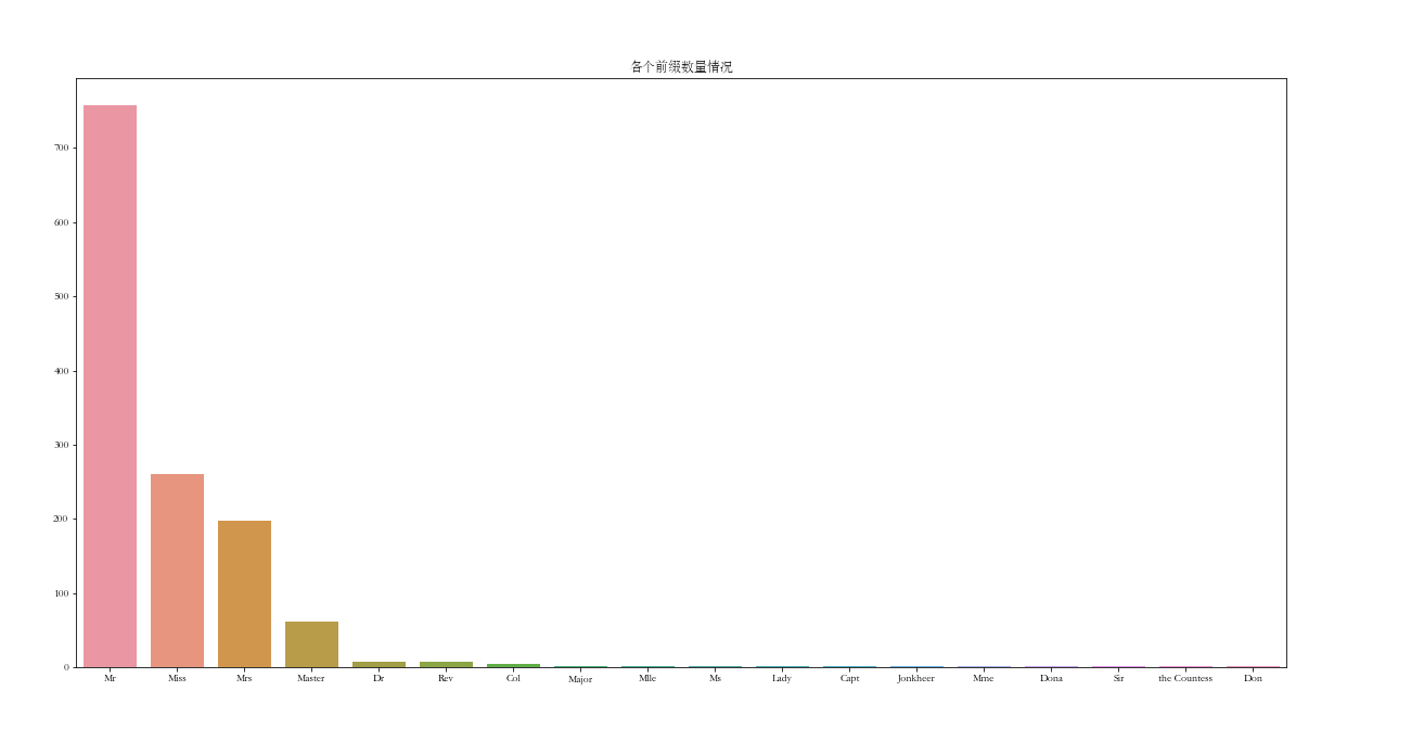
Here, I put the common Mr, Miss, Mrs and Ms into one category, and the others into one category
df_all['Title'].replace(['Mr','Miss','Mrs','Ms'],'cate1',inplace=True)
df_all['Title'] = df_all['Title'].apply(lambda x:'cate1' if x=='cate1' else 'cate2')
df_all['Title'].value_counts()
cate1    1216
cate2      93
Name: Title, dtype: int64
cate1 stands for Mr, Miss, Mrs and Ms, and cate2 stands for others
df_all[:3]
| PassengerId | Survived | Pclass | Name | Sex | Age | SibSp | Parch | Ticket | Fare | Cabin | Embarked | Family_Size | Title | |
|---|---|---|---|---|---|---|---|---|---|---|---|---|---|---|
| 0 | 1 | 0.0 | 3 | Braund, Mr. Owen Harris | male | 22.0 | 1 | 0 | A/5 21171 | 7.2500 | M | S | 2 | cate1 |
| 1 | 2 | 1.0 | 1 | Cumings, Mrs. John Bradley (Florence Briggs Th... | female | 38.0 | 1 | 0 | PC 17599 | 71.2833 | C | C | 2 | cate1 |
| 2 | 3 | 1.0 | 3 | Heikkinen, Miss. Laina | female | 26.0 | 0 | 0 | STON/O2. 3101282 | 7.9250 | M | S | 1 | cate1 |
Delete feature --- passengerid, name, ticket
df_all.drop(columns=['PassengerId','Name','Ticket'],inplace=True)
df_all[:3]
| Survived | Pclass | Sex | Age | SibSp | Parch | Fare | Cabin | Embarked | Family_Size | Title | |
|---|---|---|---|---|---|---|---|---|---|---|---|
| 0 | 0.0 | 3 | male | 22.0 | 1 | 0 | 7.2500 | M | S | 2 | cate1 |
| 1 | 1.0 | 1 | female | 38.0 | 1 | 0 | 71.2833 | C | C | 2 | cate1 |
| 2 | 1.0 | 3 | female | 26.0 | 0 | 0 | 7.9250 | M | S | 1 | cate1 |
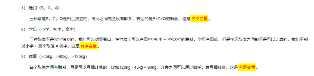
Classification feature coding
Nominal variable and distance variable are suitable for OneHotEncoder
Distance variable, suitable for LabelEncoder
df_all
| Survived | Pclass | Sex | Age | SibSp | Parch | Fare | Cabin | Embarked | Family_Size | Title | |
|---|---|---|---|---|---|---|---|---|---|---|---|
| 0 | 0.0 | 3 | male | 22.0 | 1 | 0 | 7.2500 | M | S | 2 | cate1 |
| 1 | 1.0 | 1 | female | 38.0 | 1 | 0 | 71.2833 | C | C | 2 | cate1 |
| 2 | 1.0 | 3 | female | 26.0 | 0 | 0 | 7.9250 | M | S | 1 | cate1 |
| 3 | 1.0 | 1 | female | 35.0 | 1 | 0 | 53.1000 | C | S | 2 | cate1 |
| 4 | 0.0 | 3 | male | 35.0 | 0 | 0 | 8.0500 | M | S | 1 | cate1 |
| ... | ... | ... | ... | ... | ... | ... | ... | ... | ... | ... | ... |
| 1304 | NaN | 3 | male | 28.0 | 0 | 0 | 8.0500 | M | S | 1 | cate1 |
| 1305 | NaN | 1 | female | 39.0 | 0 | 0 | 108.9000 | C | C | 1 | cate2 |
| 1306 | NaN | 3 | male | 38.5 | 0 | 0 | 7.2500 | M | S | 1 | cate1 |
| 1307 | NaN | 3 | male | 28.0 | 0 | 0 | 8.0500 | M | S | 1 | cate1 |
| 1308 | NaN | 3 | male | 36.0 | 1 | 1 | 22.3583 | M | C | 3 | cate2 |
1309 rows × 11 columns
Sex,Cabin,Embarked,Title
The four feature s to be encoded here should be encoded with onehot
OneHotEncoder
cat_features_list = ['Sex', 'Cabin', 'Embarked', 'Title']
df_all_encode = pd.DataFrame()
for feature in cat_features_list:
    data_encode = OneHotEncoder().fit_transform(df_all[feature].values.reshape(-1, 1)).toarray()
    value_count = df_all[feature].unique().size
    new_columns = ['{}_{}'.format(feature,i) for i in range(1,value_count+1)]
    print(new_columns)
    df_encode = pd.DataFrame(data_encode,columns=new_columns)
#     print(df_encode)
    df_all_encode = pd.concat([df_all_encode,df_encode],axis=1)
['Sex_1', 'Sex_2']
['Cabin_1', 'Cabin_2', 'Cabin_3', 'Cabin_4', 'Cabin_5', 'Cabin_6', 'Cabin_7', 'Cabin_8', 'Cabin_9']
['Embarked_1', 'Embarked_2', 'Embarked_3']
['Title_1', 'Title_2']
The data encoded by OneHotEncoder is as follows
df_all_encode
| Sex_1 | Sex_2 | Cabin_1 | Cabin_2 | Cabin_3 | Cabin_4 | Cabin_5 | Cabin_6 | Cabin_7 | Cabin_8 | Cabin_9 | Embarked_1 | Embarked_2 | Embarked_3 | Title_1 | Title_2 | |
|---|---|---|---|---|---|---|---|---|---|---|---|---|---|---|---|---|
| 0 | 0.0 | 1.0 | 0.0 | 0.0 | 0.0 | 0.0 | 0.0 | 0.0 | 0.0 | 1.0 | 0.0 | 0.0 | 0.0 | 1.0 | 1.0 | 0.0 |
| 1 | 1.0 | 0.0 | 0.0 | 0.0 | 1.0 | 0.0 | 0.0 | 0.0 | 0.0 | 0.0 | 0.0 | 1.0 | 0.0 | 0.0 | 1.0 | 0.0 |
| 2 | 1.0 | 0.0 | 0.0 | 0.0 | 0.0 | 0.0 | 0.0 | 0.0 | 0.0 | 1.0 | 0.0 | 0.0 | 0.0 | 1.0 | 1.0 | 0.0 |
| 3 | 1.0 | 0.0 | 0.0 | 0.0 | 1.0 | 0.0 | 0.0 | 0.0 | 0.0 | 0.0 | 0.0 | 0.0 | 0.0 | 1.0 | 1.0 | 0.0 |
| 4 | 0.0 | 1.0 | 0.0 | 0.0 | 0.0 | 0.0 | 0.0 | 0.0 | 0.0 | 1.0 | 0.0 | 0.0 | 0.0 | 1.0 | 1.0 | 0.0 |
| ... | ... | ... | ... | ... | ... | ... | ... | ... | ... | ... | ... | ... | ... | ... | ... | ... |
| 1304 | 0.0 | 1.0 | 0.0 | 0.0 | 0.0 | 0.0 | 0.0 | 0.0 | 0.0 | 1.0 | 0.0 | 0.0 | 0.0 | 1.0 | 1.0 | 0.0 |
| 1305 | 1.0 | 0.0 | 0.0 | 0.0 | 1.0 | 0.0 | 0.0 | 0.0 | 0.0 | 0.0 | 0.0 | 1.0 | 0.0 | 0.0 | 0.0 | 1.0 |
| 1306 | 0.0 | 1.0 | 0.0 | 0.0 | 0.0 | 0.0 | 0.0 | 0.0 | 0.0 | 1.0 | 0.0 | 0.0 | 0.0 | 1.0 | 1.0 | 0.0 |
| 1307 | 0.0 | 1.0 | 0.0 | 0.0 | 0.0 | 0.0 | 0.0 | 0.0 | 0.0 | 1.0 | 0.0 | 0.0 | 0.0 | 1.0 | 1.0 | 0.0 |
| 1308 | 0.0 | 1.0 | 0.0 | 0.0 | 0.0 | 0.0 | 0.0 | 0.0 | 0.0 | 1.0 | 0.0 | 1.0 | 0.0 | 0.0 | 0.0 | 1.0 |
1309 rows × 16 columns
Splice the data generated by OneHotEncoder encoding and df_all, and delete the four feature s before encoding: ['Sex', 'Cabin', 'embanked', 'Title']
df_all = pd.concat([df_all,df_all_encode],axis=1)
df_all.drop(columns=['Sex','Cabin','Embarked','Title'],inplace=True)
df_all[:3]
| Survived | Pclass | Age | SibSp | Parch | Fare | Family_Size | Sex_1 | Sex_2 | Cabin_1 | ... | Cabin_5 | Cabin_6 | Cabin_7 | Cabin_8 | Cabin_9 | Embarked_1 | Embarked_2 | Embarked_3 | Title_1 | Title_2 | |
|---|---|---|---|---|---|---|---|---|---|---|---|---|---|---|---|---|---|---|---|---|---|
| 0 | 0.0 | 3 | 22.0 | 1 | 0 | 7.2500 | 2 | 0.0 | 1.0 | 0.0 | ... | 0.0 | 0.0 | 0.0 | 1.0 | 0.0 | 0.0 | 0.0 | 1.0 | 1.0 | 0.0 |
| 1 | 1.0 | 1 | 38.0 | 1 | 0 | 71.2833 | 2 | 1.0 | 0.0 | 0.0 | ... | 0.0 | 0.0 | 0.0 | 0.0 | 0.0 | 1.0 | 0.0 | 0.0 | 1.0 | 0.0 |
| 2 | 1.0 | 3 | 26.0 | 0 | 0 | 7.9250 | 1 | 1.0 | 0.0 | 0.0 | ... | 0.0 | 0.0 | 0.0 | 1.0 | 0.0 | 0.0 | 0.0 | 1.0 | 1.0 | 0.0 |
3 rows × 23 columns
df_all.info()
<class 'pandas.core.frame.DataFrame'>
RangeIndex: 1309 entries, 0 to 1308
Data columns (total 23 columns):
 #   Column       Non-Null Count  Dtype
---  ------       --------------  -----
 0   Survived     891 non-null    float64
 1   Pclass       1309 non-null   int64
 2   Age          1309 non-null   float64
 3   SibSp        1309 non-null   int64
 4   Parch        1309 non-null   int64
 5   Fare         1309 non-null   float64
 6   Family_Size  1309 non-null   int64
 7   Sex_1        1309 non-null   float64
 8   Sex_2        1309 non-null   float64
 9   Cabin_1      1309 non-null   float64
 10  Cabin_2      1309 non-null   float64
 11  Cabin_3      1309 non-null   float64
 12  Cabin_4      1309 non-null   float64
 13  Cabin_5      1309 non-null   float64
 14  Cabin_6      1309 non-null   float64
 15  Cabin_7      1309 non-null   float64
 16  Cabin_8      1309 non-null   float64
 17  Cabin_9      1309 non-null   float64
 18  Embarked_1   1309 non-null   float64
 19  Embarked_2   1309 non-null   float64
 20  Embarked_3   1309 non-null   float64
 21  Title_1      1309 non-null   float64
 22  Title_2      1309 non-null   float64
dtypes: float64(19), int64(4)
memory usage: 235.3 KB
Data segmentation
df_train = df_all.loc[:890]
df_test = df_all.loc[891:]

del df_test['Survived']
y_train = df_train['Survived'].values
del df_train['Survived']
df_train.shape
(891, 22)
df_test.shape
(418, 22)
y_train.shape
(891,)
Standardization
x_train = StandardScaler().fit_transform(df_train)
x_test = StandardScaler().fit_transform(df_test)

print('x_train shape: {}'.format(x_train.shape))
print('y_train shape: {}'.format(y_train.shape))
print('x_test shape: {}'.format(x_test.shape))
x_train shape: (891, 22)
y_train shape: (891,)
x_test shape: (418, 22)
model
Decision tree
df_result = pd.DataFrame()
from sklearn import tree
decision_tree_model = tree.DecisionTreeClassifier()
decision_tree_model.fit(x_train,y_train)
y_predict_with_dtree = decision_tree_model.predict(x_test)

df_result['y_predict_with_dtree'] = y_predict_with_dtree
df_result
| y_predict_with_dtree | |
|---|---|
| 0 | 0.0 |
| 1 | 0.0 |
| 2 | 1.0 |
| 3 | 1.0 |
| 4 | 1.0 |
| ... | ... |
| 413 | 0.0 |
| 414 | 1.0 |
| 415 | 0.0 |
| 416 | 0.0 |
| 417 | 1.0 |
418 rows × 1 columns
logistic regression
from sklearn.linear_model import LogisticRegression
lr = LogisticRegression().fit(x_train,y_train)
y_predict_with_logisticReg = lr.predict(x_test)

df_result['y_predict_with_logisticReg'] = y_predict_with_logisticReg
df_result
| y_predict_with_dtree | y_predict_with_logisticReg | |
|---|---|---|
| 0 | 0.0 | 0.0 |
| 1 | 0.0 | 0.0 |
| 2 | 1.0 | 0.0 |
| 3 | 1.0 | 0.0 |
| 4 | 1.0 | 1.0 |
| ... | ... | ... |
| 413 | 0.0 | 0.0 |
| 414 | 1.0 | 1.0 |
| 415 | 0.0 | 0.0 |
| 416 | 0.0 | 0.0 |
| 417 | 1.0 | 0.0 |
418 rows × 2 columns
Support vector machine
from sklearn import svm
svm_model = svm.SVC()
svm_model.fit(x_train,y_train)
y_predict_with_svm = svm_model.predict(x_test)

df_result['y_predict_with_svm'] = y_predict_with_svm
df_result
| y_predict_with_dtree | y_predict_with_logisticReg | y_predict_with_svm | |
|---|---|---|---|
| 0 | 0.0 | 0.0 | 0.0 |
| 1 | 0.0 | 0.0 | 1.0 |
| 2 | 1.0 | 0.0 | 0.0 |
| 3 | 1.0 | 0.0 | 0.0 |
| 4 | 1.0 | 1.0 | 0.0 |
| ... | ... | ... | ... |
| 413 | 0.0 | 0.0 | 0.0 |
| 414 | 1.0 | 1.0 | 1.0 |
| 415 | 0.0 | 0.0 | 0.0 |
| 416 | 0.0 | 0.0 | 0.0 |
| 417 | 1.0 | 0.0 | 1.0 |
418 rows × 3 columns
KNN
from sklearn import neighbors
knnmodel = neighbors.KNeighborsClassifier(n_neighbors=2) #The n_neighbors parameter is the number of classifications
knnmodel.fit(x_train,y_train)

y_predict_with_knn = knnmodel.predict(x_test)
df_result['y_predict_with_knn'] = y_predict_with_knn
df_result
| y_predict_with_dtree | y_predict_with_logisticReg | y_predict_with_svm | y_predict_with_knn | |
|---|---|---|---|---|
| 0 | 0.0 | 0.0 | 0.0 | 0.0 |
| 1 | 0.0 | 0.0 | 1.0 | 0.0 |
| 2 | 1.0 | 0.0 | 0.0 | 0.0 |
| 3 | 1.0 | 0.0 | 0.0 | 0.0 |
| 4 | 1.0 | 1.0 | 0.0 | 0.0 |
| ... | ... | ... | ... | ... |
| 413 | 0.0 | 0.0 | 0.0 | 0.0 |
| 414 | 1.0 | 1.0 | 1.0 | 1.0 |
| 415 | 0.0 | 0.0 | 0.0 | 0.0 |
| 416 | 0.0 | 0.0 | 0.0 | 0.0 |
| 417 | 1.0 | 0.0 | 1.0 | 1.0 |
418 rows × 4 columns
Random forest
from sklearn.ensemble import RandomForestClassifier
model_randomforest = RandomForestClassifier().fit(x_train,y_train)
y_predict_with_random_forest = model_randomforest.predict(x_test)
df_result['y_predict_with_random_forest'] = y_predict_with_random_forest
df_result
| y_predict_with_dtree | y_predict_with_logisticReg | y_predict_with_svm | y_predict_with_knn | y_predict_with_random_forest | |
|---|---|---|---|---|---|
| 0 | 0.0 | 0.0 | 0.0 | 0.0 | 0.0 |
| 1 | 0.0 | 0.0 | 1.0 | 0.0 | 0.0 |
| 2 | 1.0 | 0.0 | 0.0 | 0.0 | 0.0 |
| 3 | 1.0 | 0.0 | 0.0 | 0.0 | 0.0 |
| 4 | 1.0 | 1.0 | 0.0 | 0.0 | 0.0 |
| ... | ... | ... | ... | ... | ... |
| 413 | 0.0 | 0.0 | 0.0 | 0.0 | 0.0 |
| 414 | 1.0 | 1.0 | 1.0 | 1.0 | 1.0 |
| 415 | 0.0 | 0.0 | 0.0 | 0.0 | 0.0 |
| 416 | 0.0 | 0.0 | 0.0 | 0.0 | 0.0 |
| 417 | 1.0 | 0.0 | 1.0 | 1.0 | 1.0 |
418 rows × 5 columns
Result verification
Here, in order to quickly obtain the accuracy of my prediction data locally, I obtained the prediction results with 100% accuracy from the records submitted by other gods of kaggle as the verification data;
Therefore, the accuracy of the above five models is as follows, and the random forest score is the highest: 0.7871.
df_check = pd.read_csv(r'../titanic_dir/titanic_data/correct_submission_titanic.csv')
df_check = df_check['Survived']
# df_check
for column in df_result:
    df_concat = pd.concat([df_result[column],df_check],axis=1)
    df_concat['predict_tag'] = df_concat.apply(lambda x: 1 if x[0]==x[1] else 0,axis=1)
    right_rate = df_concat['predict_tag'].sum()/df_concat['predict_tag'].count()
    print(column,'The accuracy is:')
    print(np.round(right_rate,4))
y_predict_with_dtree The accuracy is:
0.7057
y_predict_with_logisticReg The accuracy is:
0.7703
y_predict_with_svm The accuracy is:
0.7656
y_predict_with_knn The accuracy is:
0.7656
y_predict_with_random_forest The accuracy is:
0.7871
Result regression optimization
1
When filling in the missing value, Bin: the Cabin has only been dealt with briefly, and there is no good analysis on how to deal with it. I feel that different positions of the Cabin still have a great impact on the probability of being rescued. Moreover, the proportion of missing values of this attribute is very large, and the method of missing value treatment should have a great impact on the results. When optimizing later, we should spend more time thinking about how to do it ;
2
When you call the model, you simply call the five models without selecting some parameters. During later optimization, you can filter the parameters for each model, and then predict. The results should be much better.