preface
Some time ago, the leader suddenly called me to the office
The senior management of the company should take a look at the performance data analysis of the project team in the first half of the year, and get ready! All right?
I can't help it. I have to be tough! Promise and guarantee to complete the task!
When it comes to data analysis, it must be inseparable from data visualization. After all, charts are more intuitive than cold numbers. Boss can see the trend and conclusion at a glance.
Today, let's talk about some common charts in pyecharts.

install
First of all, we need to install pyecarts, which can be installed directly through pip instruction.
pip install pyecharts
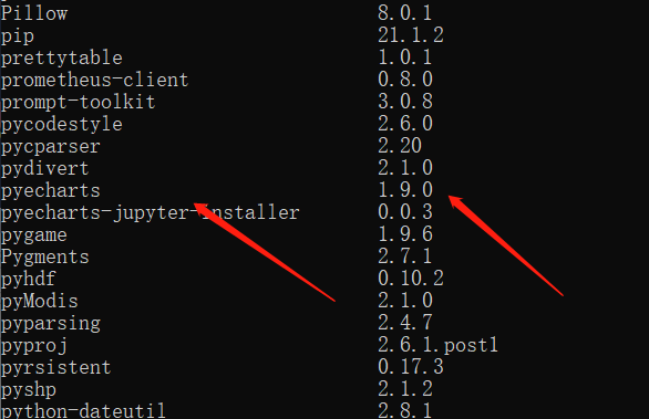
After installation, you can view the list of libraries installed by python through the pip list command. Check the installed version of pyecarts and whether the installation is successful.
Import module
As the old rule, for the smooth development of the story, we can first import the modules required in this article.
from pyecharts.charts import Bar
from pyecharts.charts import Pie
from pyecharts.charts import Line
from pyecharts import options as opts
from pyecharts.charts import EffectScatter
from pyecharts.globals import SymbolType
from pyecharts.charts import Grid
from pyecharts.charts import WordCloud
from pyecharts.charts import Map
import random
Note: the following charts are generated in the Jupyter Notebook environment.
Histogram
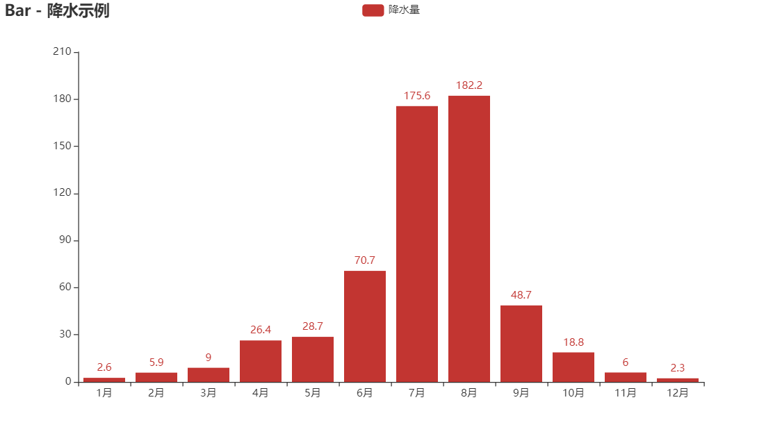
At ordinary times, what we see most is the histogram. It is also very simple for pyecharts to generate the histogram. Just fill in the data of x-axis and y-axis directly.
x = ['1 month', '2 month', '3 month', '4 month', '5 month', '6 month', '7 month', '8 month', '9 month', '10 month', '11 month', '12 month']
data_china = [2.6, 5.9, 9.0, 26.4, 28.7, 70.7, 175.6, 182.2, 48.7, 18.8, 6.0, 2.3]
data_russia = [1.6, 5.4, 9.3, 28.4, 22.7, 60.7, 162.6, 199.2, 56.7, 43.8, 3.0, 4.9]

bar = Bar()
bar.add_xaxis(x)
bar.add_yaxis("precipitation", data_china)
bar.set_global_opts(title_opts=opts.TitleOpts(title="Bar - Precipitation example"))
bar.rerender_notebook()
After run ning the program, you will get the histogram as follows:
Of course, pyecharts also supports chain call, and the functions are the same. The code is as follows:
bar = (
    Bar()
    .add_xaxis(x)
    .add_yaxis('china', data_china)
    .set_global_opts(title_opts=opts.TitleOpts(title="Bar - Precipitation example"))
)
bar.render_notebook()
In addition, you can also add multiple y-axis records to a histogram to realize multiple columnar comparison. You only need to call add one more time_ Yaxis is enough.
bar = (
    Bar()
    .add_xaxis(x)
    .add_yaxis('china', data_china)
    .add_yaxis("sussia", data_russia)
    .set_global_opts(title_opts=opts.TitleOpts(title="Bar - Multi histogram"))
)
bar.render_notebook()

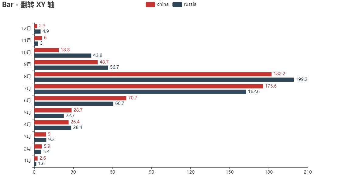
Sometimes, the histogram is too high and inconvenient to see. We can also exchange the x-axis and y-axis to generate a horizontal histogram. The multi histogram and xy axis are interchangeable without conflict and can be superimposed.
bar = (
    Bar()
    .add_xaxis(x)
    .add_yaxis('china', data_china)
    .add_yaxis('russia', data_russia)
    .reversal_axis()
    .set_series_opts(label_opts=opts.LabelOpts(position="right"))
    .set_global_opts(title_opts=opts.TitleOpts(title="Bar - Flip XY axis"))
)
bar.render_notebook()
Pie chart
Pie chart is also one of the charts with high frequency of use, especially the chart applicable to percentage category, which can intuitively see the proportion of the overall share of each category.
pie = (
    Pie()
    .add("", [list(z) for z in zip(x, data_china)])
    .set_global_opts(title_opts=opts.TitleOpts(title="Pie chart example"))
    .set_series_opts(label_opts=opts.LabelOpts(formatter="{b}: {c}"))
)
pie.render_notebook()

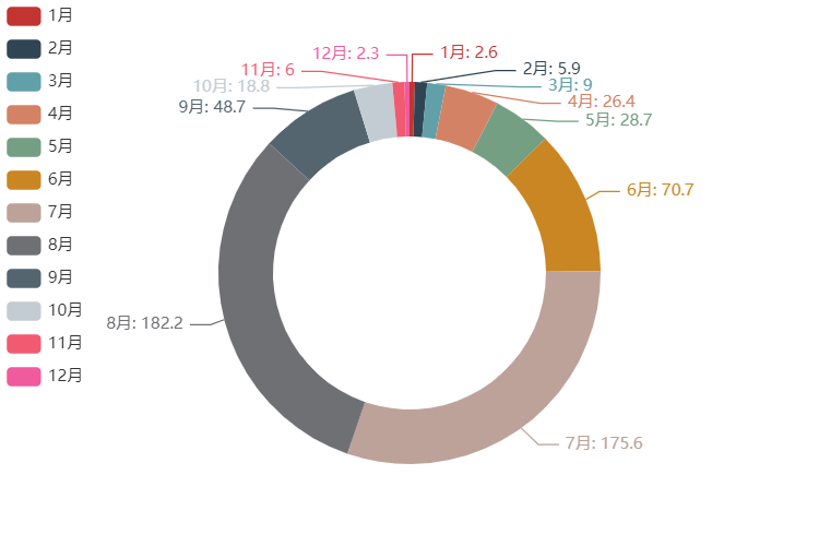
Circular pie chart
pie = (
    Pie(init_opts=opts.InitOpts(width="600px", height="400px"))
    .add(
        series_name="rainfall",
        data_pair=[list(z) for z in zip(x, data_china)],
        radius=["50%", "70%"],
        label_opts=opts.LabelOpts(is_show=False, position="center"),
    )
    .set_global_opts(legend_opts=opts.LegendOpts(pos_left="legft", orient="vertical"))
    .set_series_opts(
        tooltip_opts=opts.TooltipOpts(
            trigger="item", formatter="{a} <br/>{b}: {c} ({d}%)"
        ),
    label_opts=opts.LabelOpts(formatter="{b}: {c}")
    )
)
pie.render_notebook()
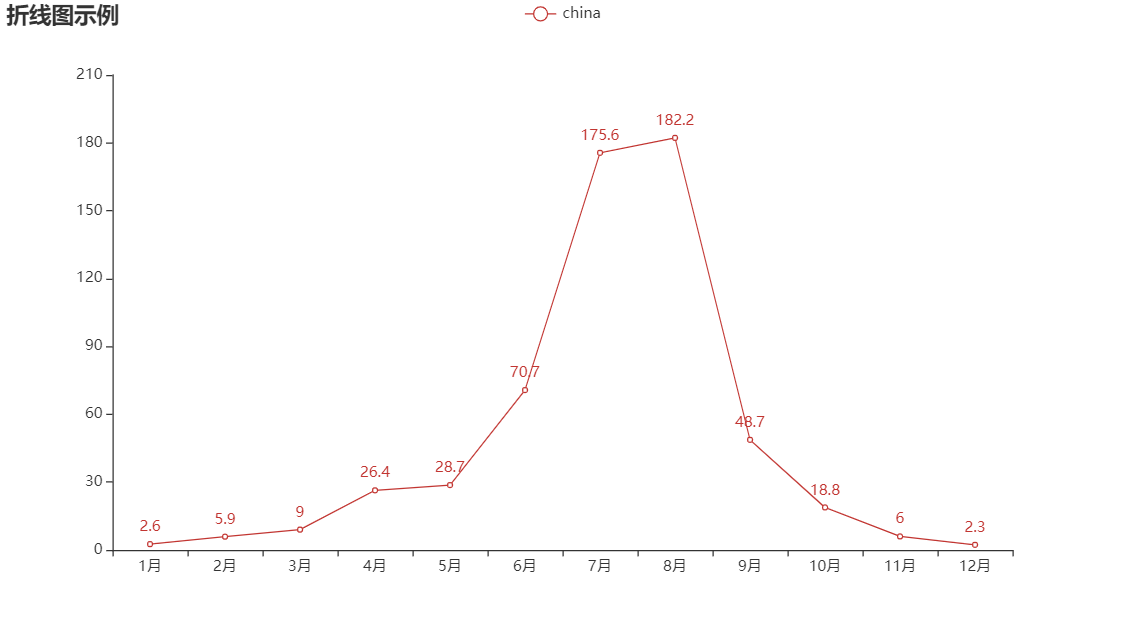
Line chart
The line chart is usually used to show the trend of data in different time periods. For example, the classic stock market K-line chart is one of the line charts.
line = (
    Line()
    .add_xaxis(x)
    .add_yaxis('china', data_china)
    .set_global_opts(title_opts=opts.TitleOpts(title="Line chart example"))
)
line.render_notebook()
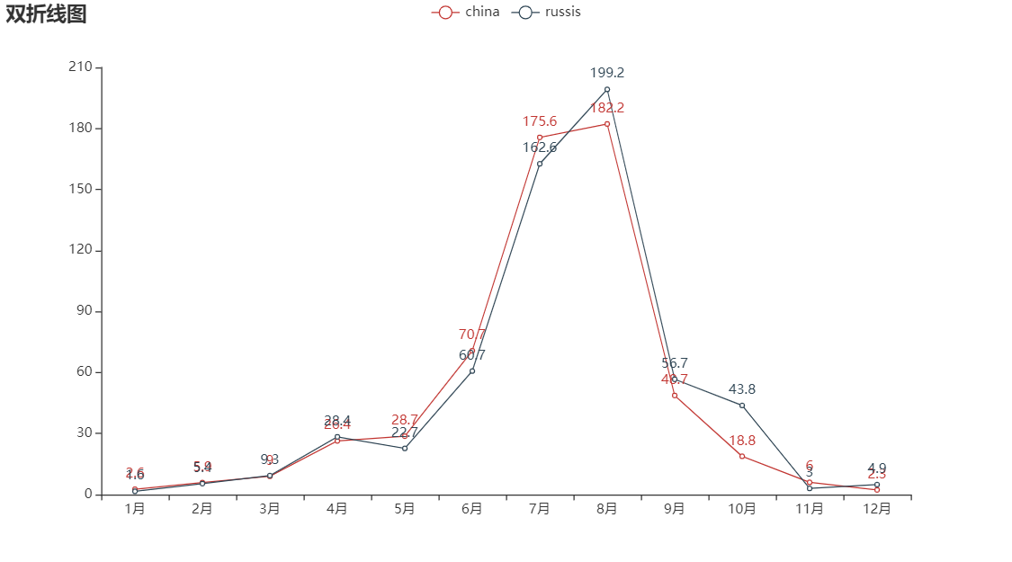
Similarly, like a bar chart, a line chart can also add multiple y-axis records to a chart.
line = (
    Line()
    .add_xaxis(x)
    .add_yaxis('china', data_china)
    .add_yaxis('russis', data_russia)
    .set_global_opts(title_opts=opts.TitleOpts(title="Double line chart"))
)
line.render_notebook()
Of course, there is also a step line chart, which can also be realized.
line = (
    Line()
    .add_xaxis(x)
    .add_yaxis('china', data_china, is_step=True)
    .set_global_opts(title_opts=opts.TitleOpts(title="Step line chart"))
)
line.render_notebook()

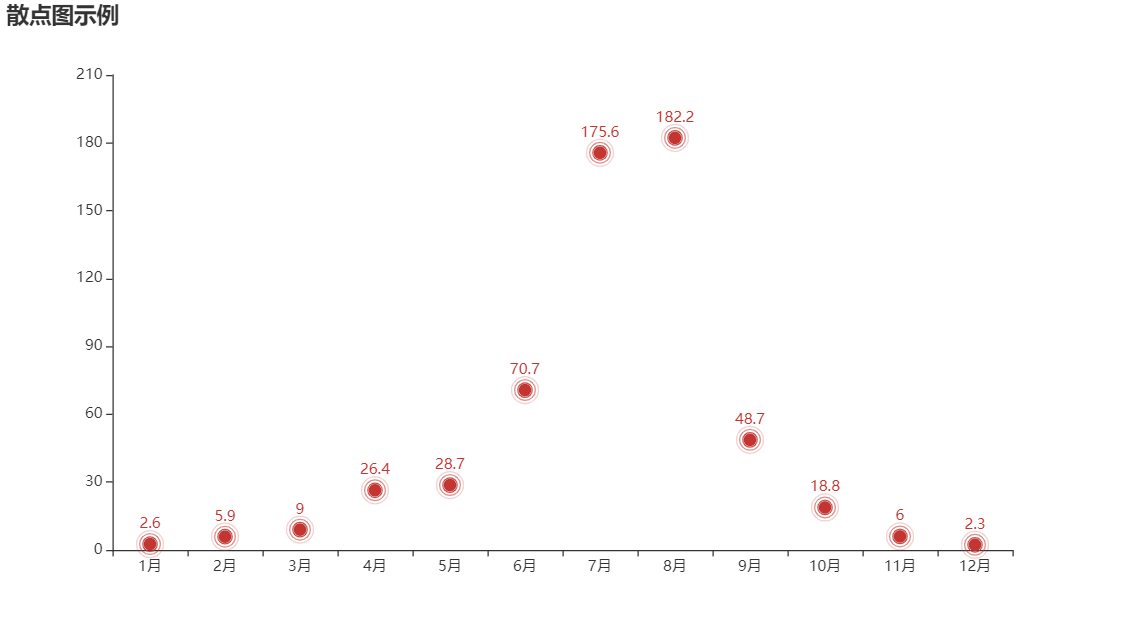
Scatter diagram
scatter = (
    EffectScatter()
    .add_xaxis(x)
    .add_yaxis("", data_china)
    .set_global_opts(title_opts=opts.TitleOpts(title="Scatter chart example"))
)
scatter.render_notebook()
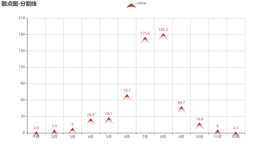
The data comparison is not very clear. We can add grid to the scatter diagram to make the y-axis data corresponding to each point more visible.
scatter = (
    EffectScatter()
    .add_xaxis(x)
    .add_yaxis("china", data_china, symbol=SymbolType.ARROW)
    .set_global_opts(
        title_opts=opts.TitleOpts(title="Scatter diagram-Split line"),
        xaxis_opts=opts.AxisOpts(splitline_opts=opts.SplitLineOpts(is_show=True)),
        yaxis_opts=opts.AxisOpts(splitline_opts=opts.SplitLineOpts(is_show=True)),
    )
)
scatter.render_notebook()
We can also specify the shape of points and add multiple y-axis records to a scatter chart. These configurations are stacked like building blocks.
scatter = (
    EffectScatter()
    .add_xaxis(x)
    .add_yaxis("china", [x + 30 for x in data_russia],symbol=SymbolType.ARROW)
    .add_yaxis("russia", data_russia, symbol=SymbolType.TRIANGLE)
    .set_global_opts(
        title_opts=opts.TitleOpts(title="Split line-Scatter diagram"),
        xaxis_opts=opts.AxisOpts(splitline_opts=opts.SplitLineOpts(is_show=True)),
        yaxis_opts=opts.AxisOpts(splitline_opts=opts.SplitLineOpts(is_show=True)),
    )
)
scatter.render_notebook()

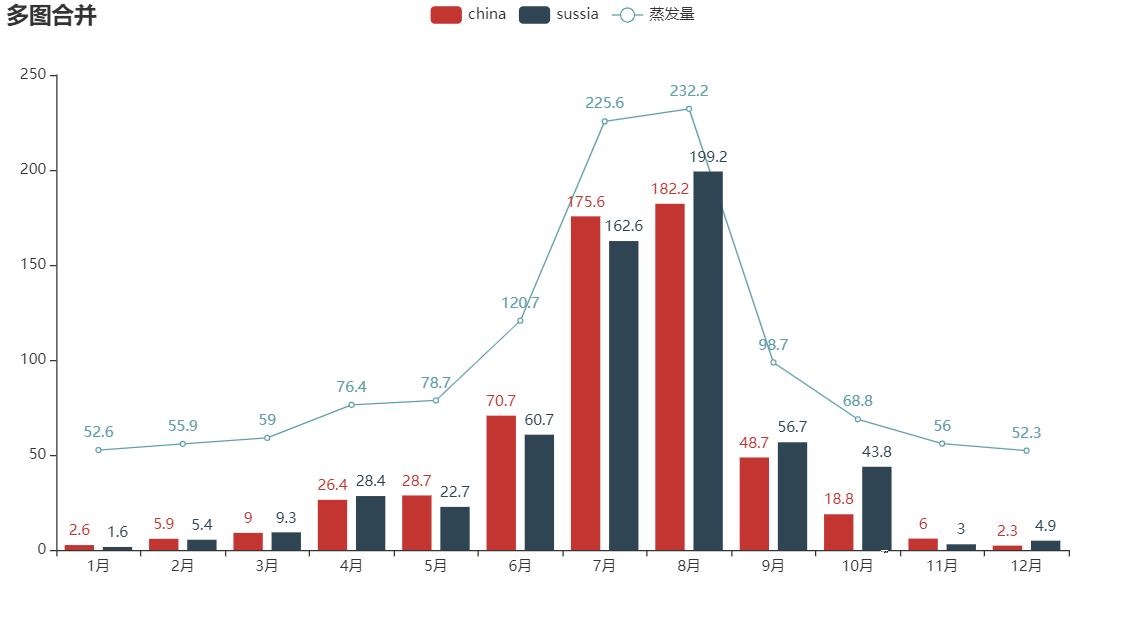
Chart merge
Sometimes, we have to put many kinds of pictures on one picture to display them, and pyechars also thought of it. The basic step is to generate the graphs of each category separately, and then combine the two with Grid.
For example, if we want to put the Bar chart and Line chart together, we should first generate Bar and Line respectively, and then combine them.
from pyecharts.charts import Grid

bar = (
    Bar()
    .add_xaxis(x)
    .add_yaxis('china', data_china)
    .add_yaxis("sussia", data_russia)
    .set_global_opts(
        title_opts=opts.TitleOpts(title="Multi graph merging"),
    )
)

line = (
    Line()
    .add_xaxis(x)
    .add_yaxis("Evaporation capacity", [x + 50 for x in data_china]
    )
)

bar.overlap(line)
grid = Grid()
grid.add(bar, opts.GridOpts(pos_left="5%", pos_right="5%"), is_control_axis_index=True)
grid.render_notebook()
Ci Yun
pyechars is also OK for word cloud. There is no problem with Chinese and there will be no garbled code.
import pyecharts.options as opts
from pyecharts.charts import WordCloud

data = [("Living resources", "999"),("Heating management", "888"),("Gas supply quality", "777"),("Domestic water management", "688"),("Primary water supply", "588"),("Transportation", "516"),("Urban transportation", "515"),("environmental protection", "483"),("Real estate management", "462"),("Urban and rural construction", "449"),("Social security and welfare", "429"),("social security", "407"),("Sports and educational management", "406"),("Public safety", "406"),("Public transport management", "386"),("Taxi operation management", "385"),("Heating management", "375"),("City appearance and sanitation", "355"),("natural resource management ", "355"),("Dust pollution ", "335"),("noise pollution", "324"),("land resource management", "304"),("Property service and management", "304"),("medical and health work", "284"),("Fly ash pollution", "284"),("Jeeves ", "284"),("Heating development", "254"),("Rural land planning and management", "254"),("Living noise", "253"),("Influence of heating unit", "253"),("Urban power supply", "223"),("Housing quality and safety", "223"),("air pollution", "223"),("House safety", "223"),("Cultural Activity ", "223"),("Demolition management", "223"),("communal facilities", "223"),("Gas supply quality", "223"),("Power supply management", "223"),("Gas management", "152"),("education management ", "152"),("Medical disputes", "152"),("Law enforcement supervision", "152"),("Equipment safety", "152"),("Government affairs construction", "152"),("Counties, districts and development zones", "152"),("Macroeconomic", "152"),("education management ", "112"),("social security", "112"),("Domestic water management", "112"),("Property service and management", "112"),("Classification list", "112"),("agricultural production", "112"),("Secondary water supply", "112"),("Urban public facilities", "92"),("Demolition policy consultation", "92"),("Property services", "92"),("estate management", "92"),("Social security insurance management", "92"),("Subsistence management", "92"),("Entertainment market management", "72"),("Urban traffic order management", "72"),("Law enforcement disputes", "72"),("Commercial soot pollution", "72"),("Road occupation stacking", "71"),("Aboveground facilities", "71"),("Water Quality", "71"),("anhydrous", "71"),("Influence of heating unit", "71"),("Sidewalk management", "71"),("Main network reason", "71"),("Central heating", "71"),("Passenger transport management", "71"),("State owned public transport (bus) management", "71"),("Industrial dust pollution", "71"),("public security case", "71"),("Pressure vessel safety", "71"),("ID card management", "71"),("Mass fitness", "41"),("Industrial emission pollution", "41"),("Destruction of forest resources", "41"),("Market charge", "41"),("Production funds", "41"),("Production noise", "41"),("Rural subsistence allowances", "41"),("Labor dispute", "41"),("Labor contract disputes", "41"),("Labor remuneration and welfare", "41"),("malpractice", "21"),("cut off the supply", "21"),("elementary education", "21"),("vocational education", "21"),("Property qualification management", "21"),("Demolition compensation", "21"),("Facility maintenance", "21"),("Market spillover", "11"),("roadside booths", "11"),("Tree management", "11"),("Rural infrastructure", "11"),("anhydrous", "11"),("Gas supply quality", "11"),("Stop gas", "11"),("Work Department of municipal government (including department management organization and directly subordinate units)", "11"),("Gas management", "11"),("City appearance and sanitation", "11"),("News media", "11"),("Talent recruitment", "11"),("market environment", "11"),("Administrative fees", "11"),("Food safety and hygiene", "11"),("Urban transportation", "11"),("Real estate development", "11"),("Housing supporting problems", "11"),("Property services", "11"),("estate management", "11"),("Jeeves ", "11"),("Landscaping", "11"),("Registered residence management and identity card", "11"),("Public transport management", "11"),("Highway (waterway) traffic", "11"),("The house is inconsistent with the drawing", "11"),("Cable TV", "11"),("public security", "11"),("Forestry resources", "11"),("Other administrative charges", "11"),("Operating charges", "11"),("Food safety and hygiene", "11"),("Sports activities", "11"),("Cable TV installation, commissioning and maintenance", "11"),("Subsistence management", "11"),("Labor dispute", "11"),("Social welfare and affairs", "11"),("Primary water supply", "11"),]

wordCloud = (
    WordCloud()
    .add(series_name="Hot spot analysis", data_pair=data, word_size_range=[6, 66])
    .set_global_opts(
        title_opts=opts.TitleOpts(
            title="Hot spot analysis", title_textstyle_opts=opts.TextStyleOpts(font_size=23)
        ),
        tooltip_opts=opts.TooltipOpts(is_show=True),
    )
)

Map
Sometimes we want to display the data on the map, such as the national epidemic situation, the population data of all provinces, the distribution of wechat friends in all provinces, etc.
provinces = ['Guangdong', 'Beijing', 'Shanghai', 'Hunan', 'Chongqing', 'Xinjiang', 'Henan', 'Heilongjiang', 'Zhejiang', 'Taiwan']
values = [random.randint(1, 1024) for x in range(len(provinces))]

map = (
    Map()
    .add("", [list(z) for z in zip(provinces, values)], "china")
    .set_global_opts(
        title_opts=opts.TitleOpts(title="China map example"),
        visualmap_opts=opts.VisualMapOpts(max_=1024, is_piecewise=True),
    )

)
map.render_notebook()

summary
Today, we have drawn several common charts through pyecharts. Of course, drawing charts has a fixed routine process.
The generation of charts can be roughly divided into three steps: preparing relevant data, setting data and relevant configuration using chain call method, and calling render_ The notebook () or render() function generates a chart.
Well, that's all for today. Let's continue our efforts tomorrow!

Creation is not easy, white whoring is not good. Your support and recognition is the biggest driving force of my creation. See you in the next article!
Dragon youth
If there are any mistakes in this blog, please comment and advice. Thank you very much!