Main sources:
Mr. Li Mu's pytorch hands-on learning and deep learning (bow and thank you)
Record what you have learned every day. Welcome to discuss~

(the dust has finally settled in the senior year, and I am fully engaged in learning during the holiday!)

1. What is regularization?

Regularization can be translated as regularization or normalization. What are the rules? You can't check books in the closed book exam. This is the rule, a limitation. Similarly, here, regularization means adding some restrictions to the loss function, standardizing them through this rule, and then don't inflate yourself in the next cycle iteration.
See for details An article completely understands Regularization

2. Why regularization?

A simple method is through a linear function f ( x ) = w ⊤ x f(\mathbf{x}) = \mathbf{w}^\top \mathbf{x} F (x) = a norm of the weight vector in W ⊤ x to measure its complexity, e.g ∥ w ∥ 2 \| \mathbf{w} \|^2 ∥w∥2. To ensure that the weight vector is relatively small, the most common method is to add its norm as a penalty term to the problem of minimizing loss. The original training objective minimizes the prediction loss on the training label and is adjusted to minimize the sum of prediction loss and penalty term.
Now, if our weight vector grows too large, our learning algorithm may focus more on minimizing the weight norm ∥ w ∥ 2 \| \mathbf{w} \|^2 ∥w∥2. That's what we want. Our loss is given by the following formula:

L ( w , b ) = 1 n ∑ i = 1 n 1 2 ( w ⊤ x ( i ) + b − y ( i ) ) 2 . L(\mathbf{w}, b) = \frac{1}{n}\sum_{i=1}^n \frac{1}{2}\left(\mathbf{w}^\top \mathbf{x}^{(i)} + b - y^{(i)}\right)^2. L(w,b)=n1​i=1∑n​21​(w⊤x(i)+b−y(i))2.

In retrospect, x ( i ) \mathbf{x}^{(i)} x(i) is the sample i i Characteristics of i, y ( i ) y^{(i)} y(i) is the sample i i i label. ( w , b ) (\mathbf{w}, b) (w,b) are weight and bias parameters. In order to punish the size of the weight vector, we must add in some way to the loss function ∥ w ∥ 2 \| \mathbf{w} \|^2 ‖ w ‖ 2, but how should the model balance the loss of this new additional penalty? In fact, we use the regularization constant λ \lambda λ To describe this trade-off, which is a non negative hyperparameter, we use validation data to fit:

L ( w , b ) + λ 2 ∥ w ∥ 2 , L(\mathbf{w}, b) + \frac{\lambda}{2} \|\mathbf{w}\|^2, L(w,b)+2λ​∥w∥2,

about λ = 0 \lambda = 0 λ= 0, we restored the original loss function. about λ > 0 \lambda > 0 λ> 0, we limit ∥ w ∥ \| \mathbf{w} \| The size of ‖ w ‖. We still divide by 2 2 2: When we take the derivative of a quadratic function, 2 2 2 and 1 / 2 1/2 1 / 2 is offset to ensure that the update expression looks beautiful and simple. Smart readers may wonder why we use the square norm instead of the standard norm (i.e. Euclidean distance). We do this to facilitate calculation. Through square L 2 L_2 L2 ＾ norm, we remove the square root and leave the sum of squares of each component of the weight vector. This makes the penalty derivative easy to calculate: the sum of the derivatives is equal to the sum of the derivatives.

3. Code implementation

1) Generate labor dataset

%matplotlib inline
import torch
from torch import nn
from d2l import torch as d2l

The generation formula is as follows:

y = 0.05 + ∑ i = 1 d 0.01 x i + ϵ  where  ϵ ∼ N ( 0 , 0.0 1 2 ) . y = 0.05 + \sum_{i = 1}^d 0.01 x_i + \epsilon \text{ where } \epsilon \sim \mathcal{N}(0, 0.01^2). y=0.05+i=1∑d​0.01xi​+ϵ where ϵ∼N(0,0.012).

We choose that the label is a linear function of the input. The tag is destroyed by Gaussian noise with mean value of 0 and standard deviation of 0.01. In order to make the effect of over fitting more obvious, we can increase the dimension of the problem to d = 200 d = 200 d=200, and a small training set containing only 20 samples is used.

n_train, n_test, num_inputs, batch_size = 20, 100, 200, 5
true_w, true_b = torch.ones((num_inputs, 1)) * 0.01, 0.05
train_data = d2l.synthetic_data(true_w, true_b, n_train)
train_iter = d2l.load_array(train_data, batch_size)
test_data = d2l.synthetic_data(true_w, true_b, n_test)
test_iter = d2l.load_array(test_data, batch_size, is_train=False)

• When the training data is set to 20 (when the model is very complex), it is easier to over fit

2) Initialize model parameters

def init_params():
    w = torch.normal(0, 1, size=(num_inputs, 1), requires_grad=True)
    b = torch.zeros(1, requires_grad=True)
    return [w, b]

w is a vector and b is a scalar

def l2_penalty(w):
    return torch.sum(w.pow(2)) / 2

The most convenient way to achieve this penalty is to square all terms and sum them.

3) Realize

def train(lambd):
    w, b = init_params()
    net, loss = lambda X: d2l.linreg(X, w, b), d2l.squared_loss
    num_epochs, lr = 100, 0.003
    animator = d2l.Animator(xlabel='epochs', ylabel='loss', yscale='log',
                            xlim=[5, num_epochs], legend=['train', 'test'])
    for epoch in range(num_epochs):
        for X, y in train_iter:
            with torch.enable_grad():
                # L2 norm penalty term is added, and the broadcast mechanism makes l2_penalty(w) becomes a batch with a length of ` batch_size ` vector.
                l = loss(net(X), y) + lambd * l2_penalty(w)
            l.sum().backward()
            d2l.sgd([w, b], lr, batch_size)
        if (epoch + 1) % 5 == 0:
            animator.add(epoch + 1, (d2l.evaluate_loss(net, train_iter, loss),
                                     d2l.evaluate_loss(net, test_iter, loss)))
    print('w of L2 The norm is:', torch.norm(w).item())

• The first layer of loop is data iteration, and the second layer of loop is to take an x and y from the iterator each time
• Of course, there is one more lambd * l2_penalty(w), the rest are the same as before

4) Results

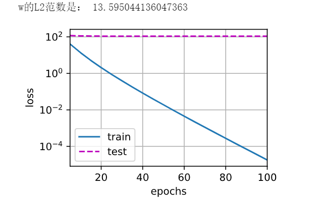
λ = 0 \lambda = 0 λ= 0: it is obviously over fitted, and the test cannot change at all

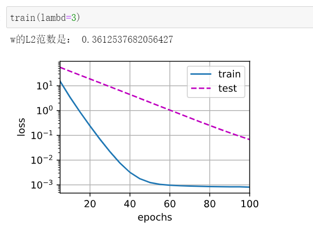
λ = 3 \lambda = 3 λ= 3: The weight is obviously smaller

5) Use framework

def train_concise(wd):
    net = nn.Sequential(nn.Linear(num_inputs, 1))
    for param in net.parameters():
        param.data.normal_()
    loss = nn.MSELoss()
    num_epochs, lr = 100, 0.003
    # The offset parameter has no attenuation.
    trainer = torch.optim.SGD([
        {"params":net[0].weight,'weight_decay': wd},
        {"params":net[0].bias}], lr=lr)
    animator = d2l.Animator(xlabel='epochs', ylabel='loss', yscale='log',
                            xlim=[5, num_epochs], legend=['train', 'test'])
    for epoch in range(num_epochs):
        for X, y in train_iter:
            with torch.enable_grad():
                trainer.zero_grad()
                l = loss(net(X), y)
            l.backward()
            trainer.step()
        if (epoch + 1) % 5 == 0:
            animator.add(epoch + 1, (d2l.evaluate_loss(net, train_iter, loss),
                                     d2l.evaluate_loss(net, test_iter, loss)))
    print('w of L2 Norm:', net[0].weight.norm().item())

• weight_decay is what we call lamda, which directly uses weight when instantiating the optimizer_ Decaly specifies the weight decaly super parameter. By default, PyTorch attenuates both weights and offsets. Here we only set the weight for the weight_decay, so the bias parameter b b b does not decay.

Summary:

• Regularization is a common method to deal with over fitting. The penalty term is added to the loss function of the training set to reduce the complexity of the learned model.
• A particular option to keep the model simple is to use L 2 L_2 L2  penalty weight attenuation. This causes weight attenuation in the learning algorithm update step.
• The weight attenuation function is provided in the optimizer of the deep learning framework.
• In the same training code implementation, different parameter sets can have different update behaviors.