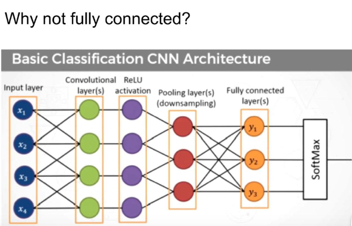
1, Convolutional neural network CNN

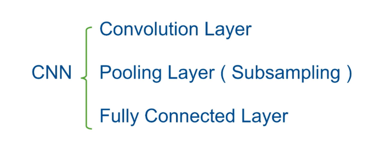
  The most classical convolutional neural network has three layers:

• Convolution Layer
• Sampling on the Pooling Layer (Subsampling)
• Fully Connected Layer

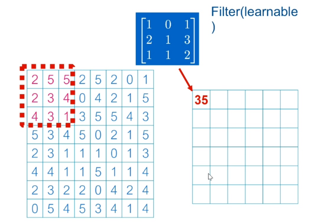
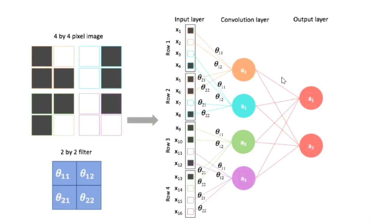
Calculation of convolution:

Matrix multiplication with the blue matrix filter in the red box, that is:

(2*1+5*0+5*1)+(2*2+3*1+4*3)+(4*1+3*1+1*2)= 35

Then move the red box back one column to continue the above calculation

Convolution neural calculation is completed to obtain the data

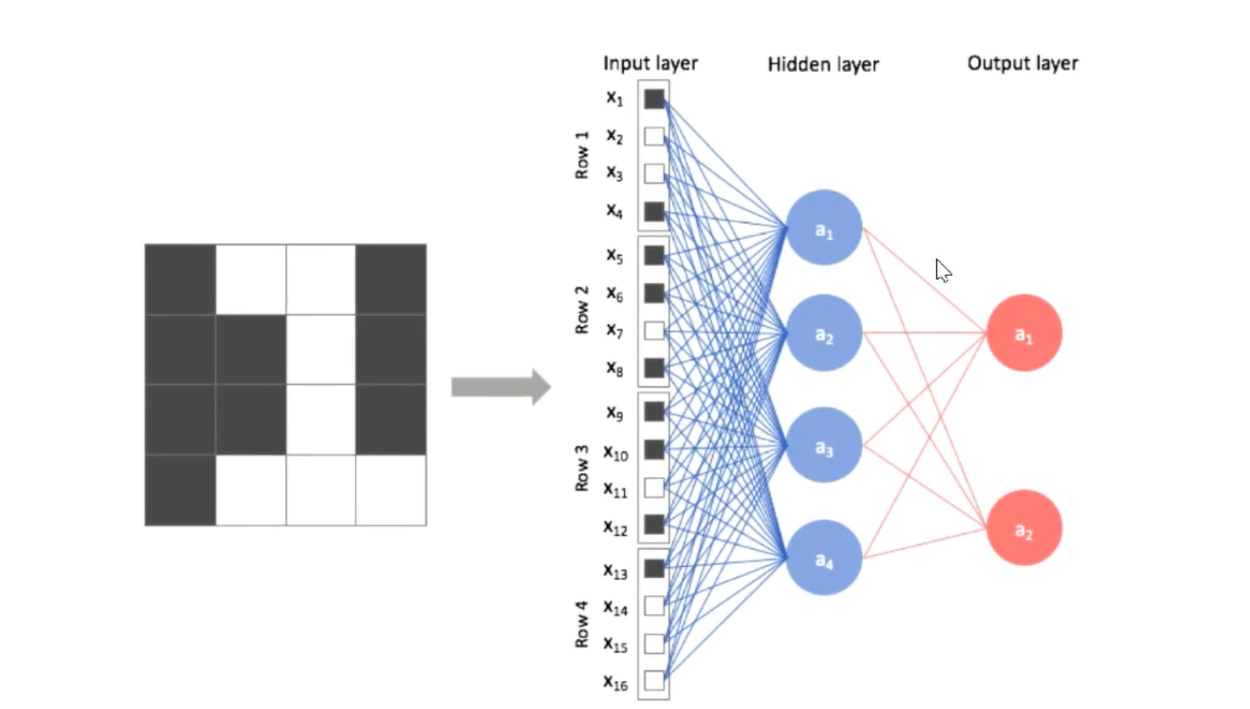
The difference between CNN and deep neural network is that CNN is not fully connected   Every data in the Filter is learned

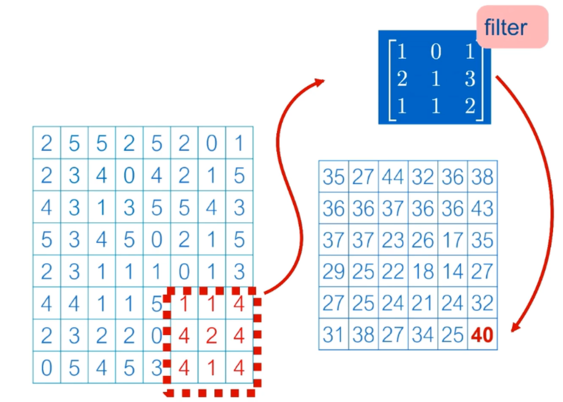
Used to extract picture features

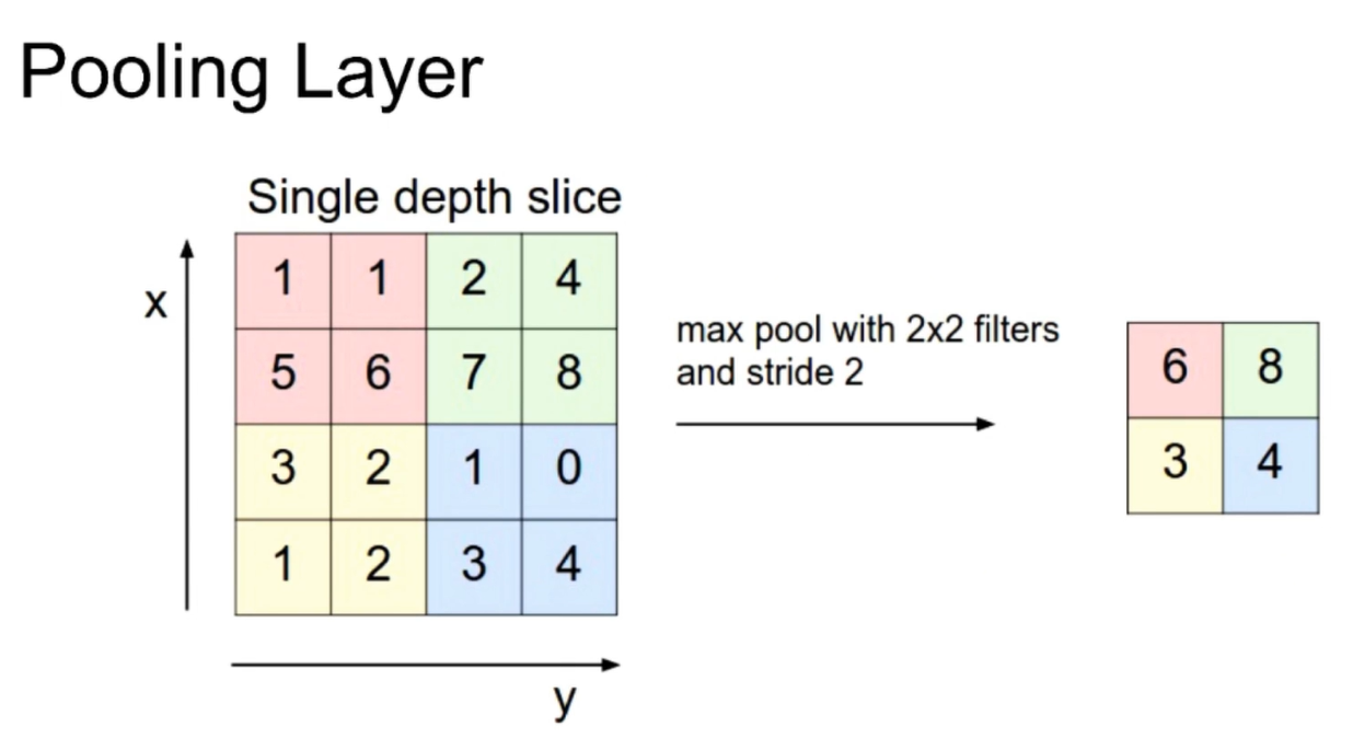
Pooling Layer

max pool goes to the largest one as the name suggests     The corresponding average pool is the average pool  

Incomplete connection

  Full connection

  Calculate loss   The back propagation method is used to transmit back, and the gradient descent method is used to reduce the error

2, Application of one-dimensional convolution

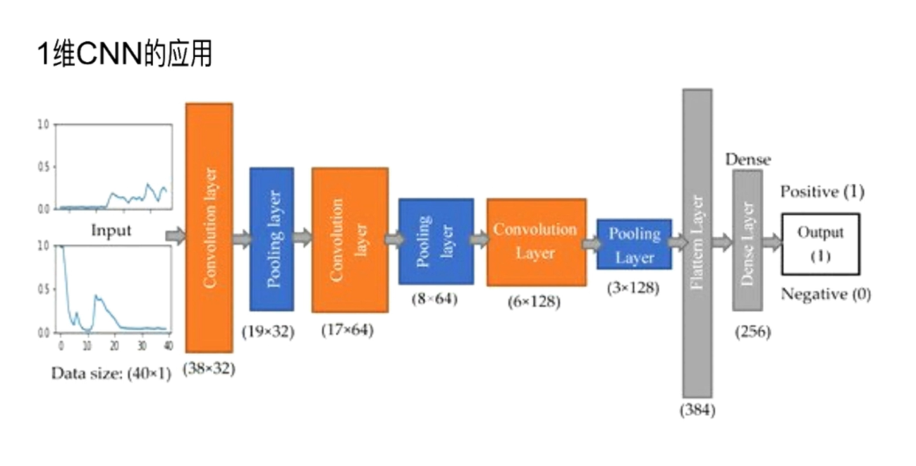
There are three layers of stock price prediction: convolution layer - pooling layer - fully connected neural network

Use the 20 day stock price to predict the stock price on the 21st day   Using mse to calculate the error between and real data

3, Code implementation

(1) Dataset preparation

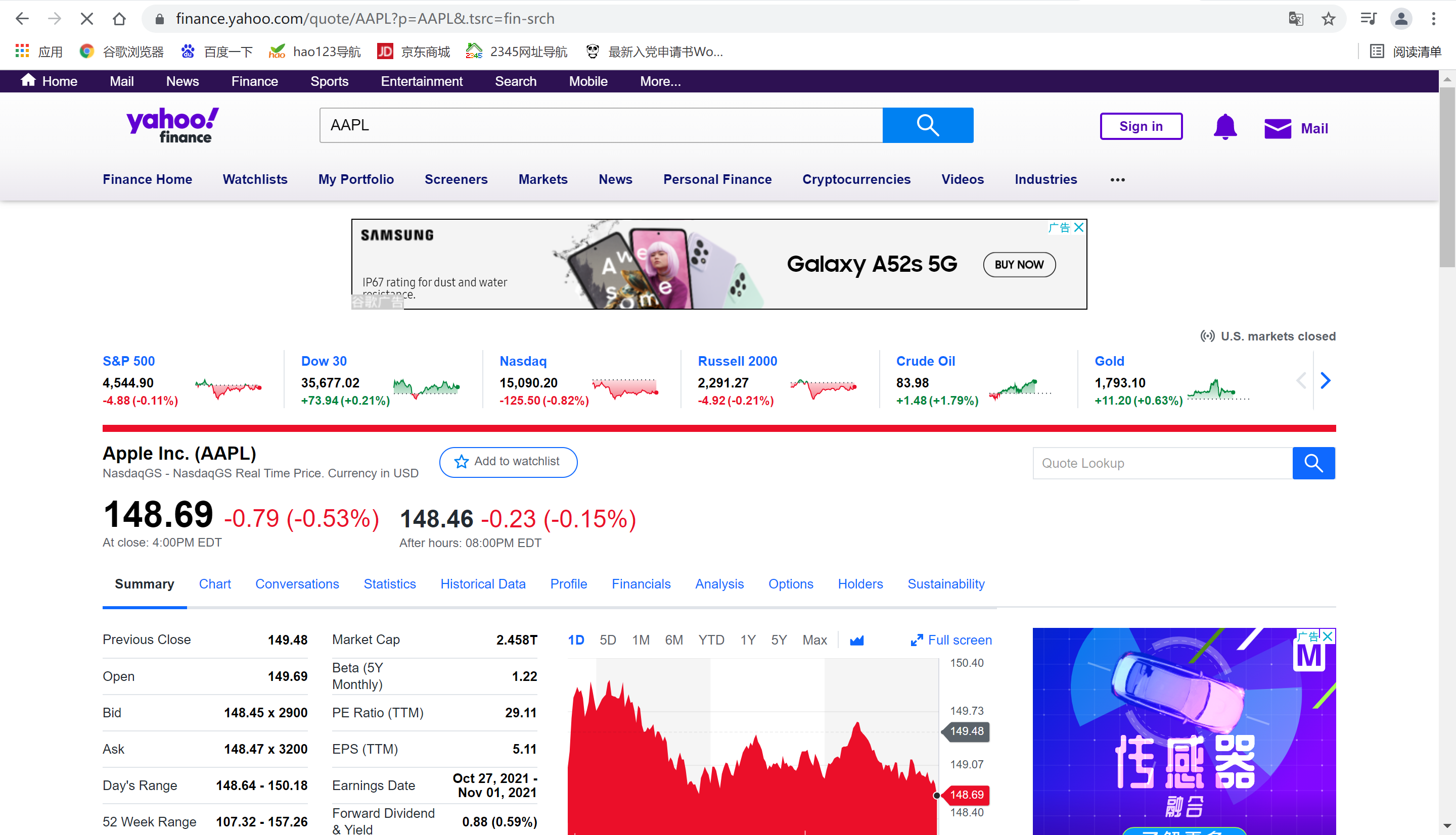
Download the data set used at finance.yaoo.com

The stock price forecast uses Apple's stock price forecast, which is directly input into AAPL search

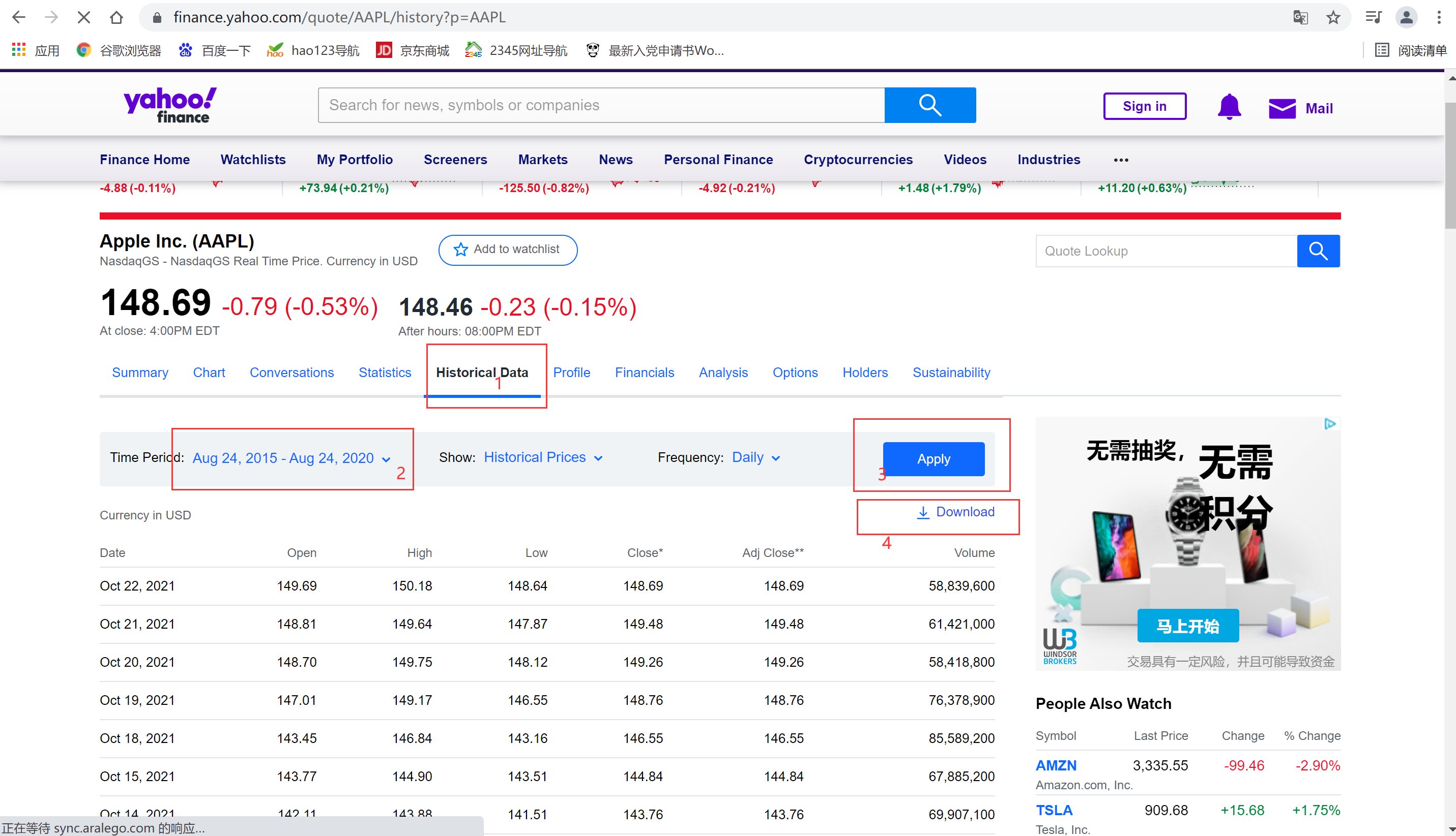  After downloading, it is a csv file. We use the stock price for 5 years   Daily closing price

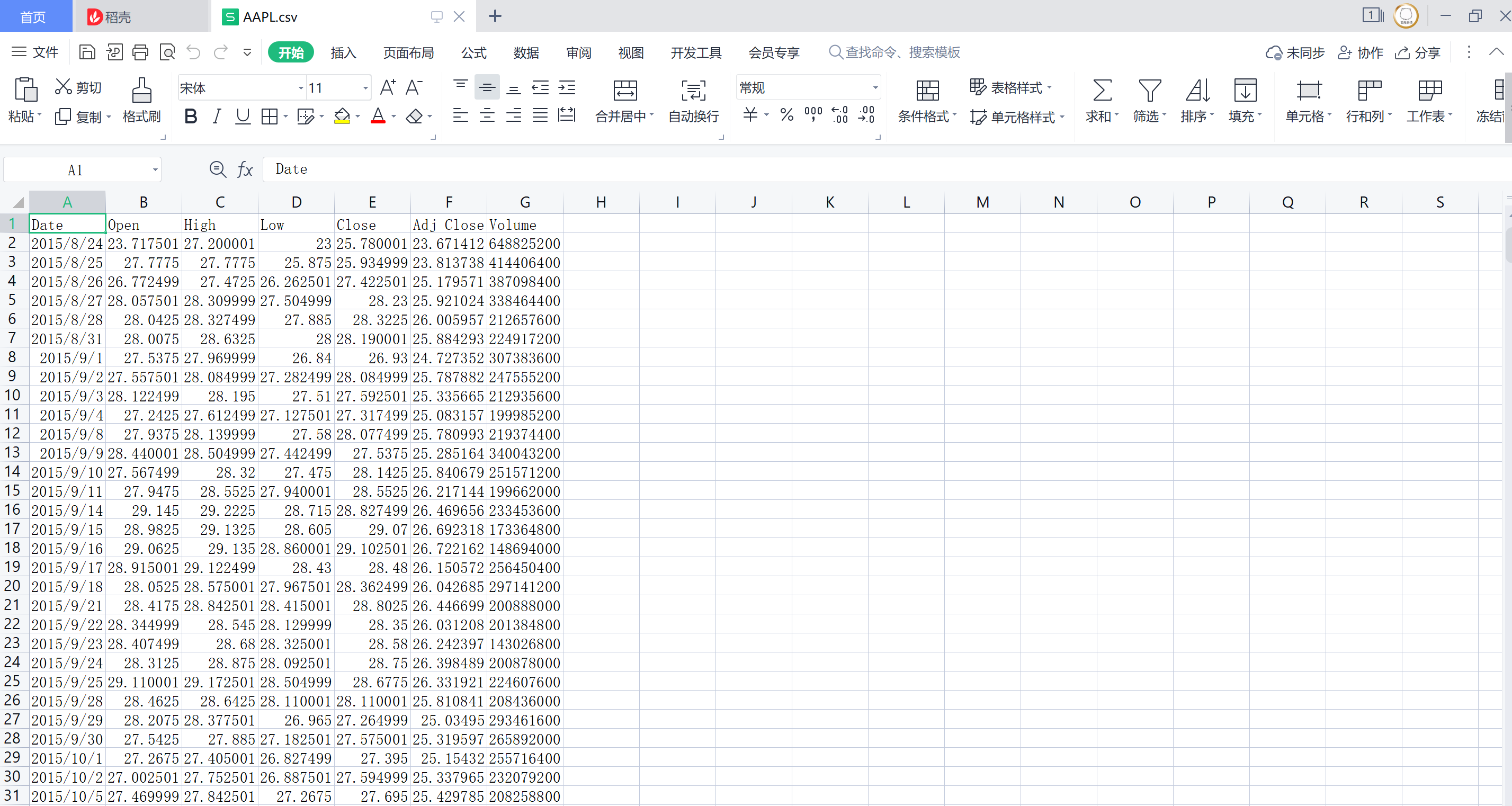
Look at our data

  (2) Code implementation

• The code running environment is based on tensorflow. This paper uses Jupiter notebook to compile the environment, and the visual results are good
• A complete code is attached at the end of the text. The meaning of each code is recorded and explained here

Use pandas to read the data and df.head() to print the first five lines of data

df = pd.read_csv('AAPL.csv')
df.head()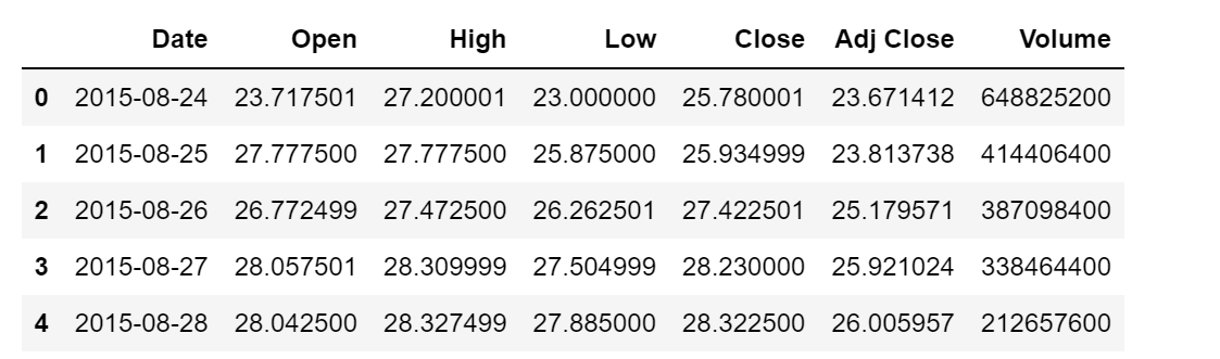

  We use the adjusted closing price Adj Close to predict the stock price. First, take out the data and save it in x0. Use the values attribute to convert it into numpy form. len(x0) will see how many data x0 has

x0 = df['Adj Close'].values
x0.shape
len(x0)

  Next, preprocess the data. We hope that each data is between 0-1, which is convenient for us to make prediction

First, we remove the largest data in x0, and then all data are divided by the largest data

x0[:10] output look at the data in x0

m = max(x0)
x0 = x0/m
x0[:10]

  n stands for the number of data, and p stands for predicting the next value with 20 data  

x is a part of the training data, from k to k+p, and k is obtained by subtracting p from the total number and adding 1

x.shape() look at the shape of X

n = len(x0)
p = 20 
x = np.array([x0[k:k+p] for k in range(n-p+1)])
x.shape

1240 pieces of data, each containing 20 pieces of data  

  Calculate y label

y = np.array(x0[p:])
y.shape

y. When shape () sees 1239 data in Y, it will find that there is one less data than x, because only the first 20 data predict a y  

  Next, adjust x so that x and y have the same data to facilitate prediction  

Because the data read by keras has three dimensions, here we add a new dimension to x to facilitate keras to read data

10. Shape () can see that X becomes three-dimensional data

X = x[:-1]
X = X[:, :, np.newaxis]
X.shape

  Split X into four parts for training and prediction,

test_size = 0.2 means that 20% of the data do training and 80% of the data do prediction

shuffle=True, let the data be re washed (when shuffle is set to False, it can be found that the prediction effect is much worse)

X_train, X_test, y_train, y_test = train_test_split(X, y, test_size=0.2, shuffle=True)

Next, build the model, mainly using Sequential in keras

The following are some packages used to build the model. Here, one-dimensional convolution and one-dimensional maximum pooling are used. I have imported two optimizers here. You can try to see the prediction effect respectively

• Dense fully connected network
• Flatten can spread two-dimensional data into one-dimensional data
• Dropout prevents overfitting
• Activate activate function

from tensorflow.keras.models import Sequential
from tensorflow.keras.layers import Dense, Flatten, Reshape, Dropout, Activation
from tensorflow.keras.layers import Conv1D, MaxPooling1D
from tensorflow.keras.optimizers import SGD
from tensorflow.keras.optimizers import Adam

The model is simple, with only three layers. One dimensional convolution layer, maximum pooling layer and flattening data are connected to a fully connected network. The activation function here uses sigmoid. (softmax is usually used for classification problems. Today's data is similar to regression problems, so sigmoid is used here.)

Model. Sumarysee the details of the model  

#Model building
model = Sequential()
#50 filter convolution kernels learn more features, and the same ensures that the dimension remains unchanged
model.add(Conv1D(50,4,padding='same',activation='relu',input_shape=(p,1))) 
model.add(MaxPooling1D(2))#Taking one big data from every two will reduce it by half
model.add(Flatten())#Turn two-dimensional data into one-dimensional data

model.add(Dense(20))#The whole connecting layer of 20 neurons
model.add(Dropout(0.2))#Prevent over fitting and 20% weight freezing
model.add(Activation('relu'))
model.add(Dense(1))#The output layer is a one-dimensional fully connected neural network
model.add(Activation('sigmoid'))

#model.compile(loss='mse',optimizer=SGD(lr=0.2), metrics['accuracy'])
model.compile(loss='mse', optimizer=SGD(lr=0.2))
model.summary()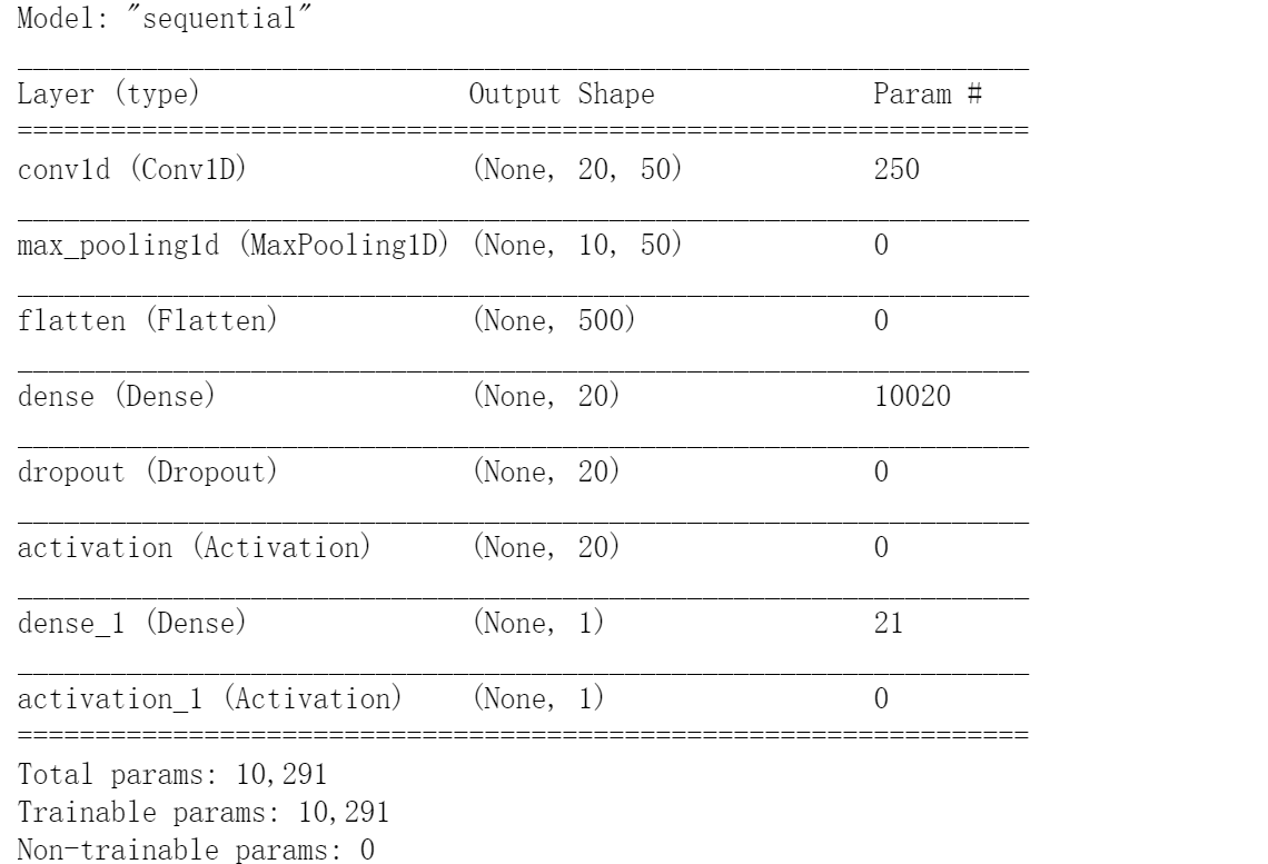

 

  Let's start training the model and use the function model.fit()

model.fit(X_train,y_train,epochs=50,batch_size=32)

  Training 50 epoch s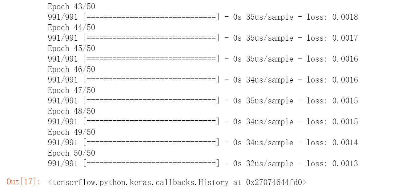

  Let's visualize the drawing data

y_predict = model.predict(X_test)
plt.plot(y_test[:100])#Take the first 100 real data
plt.plot(y_predict[:100],'r')    #Model learned

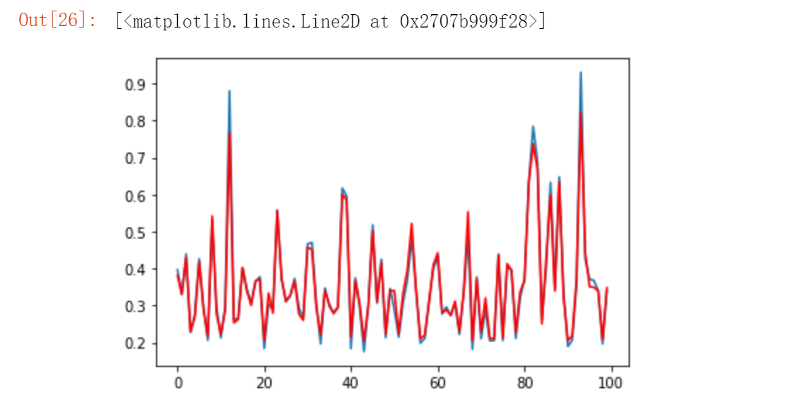
In fact, we can see that the prediction effect is still relatively good.

You can try different optimizers, activation functions, and different epoch and batch_size... Forecast results  

4, Comparison with LSTM predicted share price

Running directly down the code will make the program experience more intuitive.