The fourth chapter is the frequency domain analysis of the signal

4.1 General

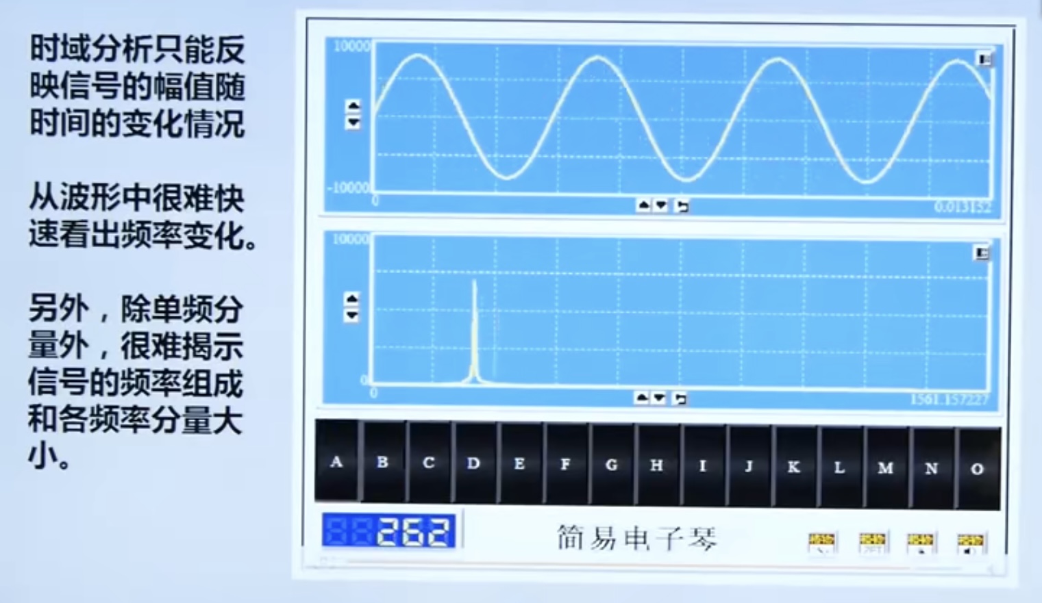
4.1. 1 limitations of time domain analysis

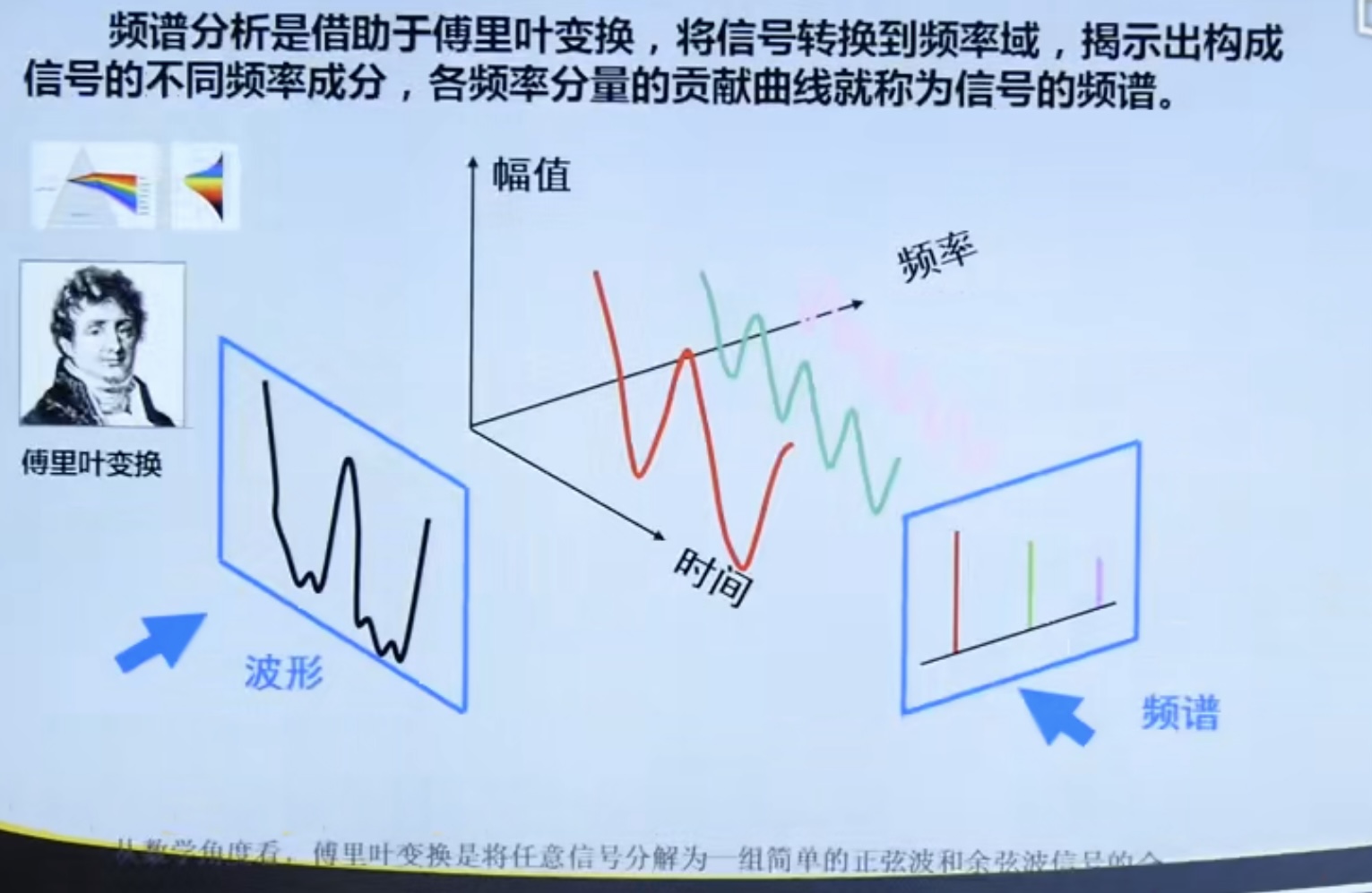
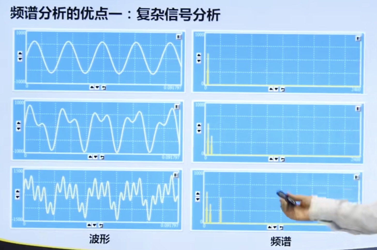
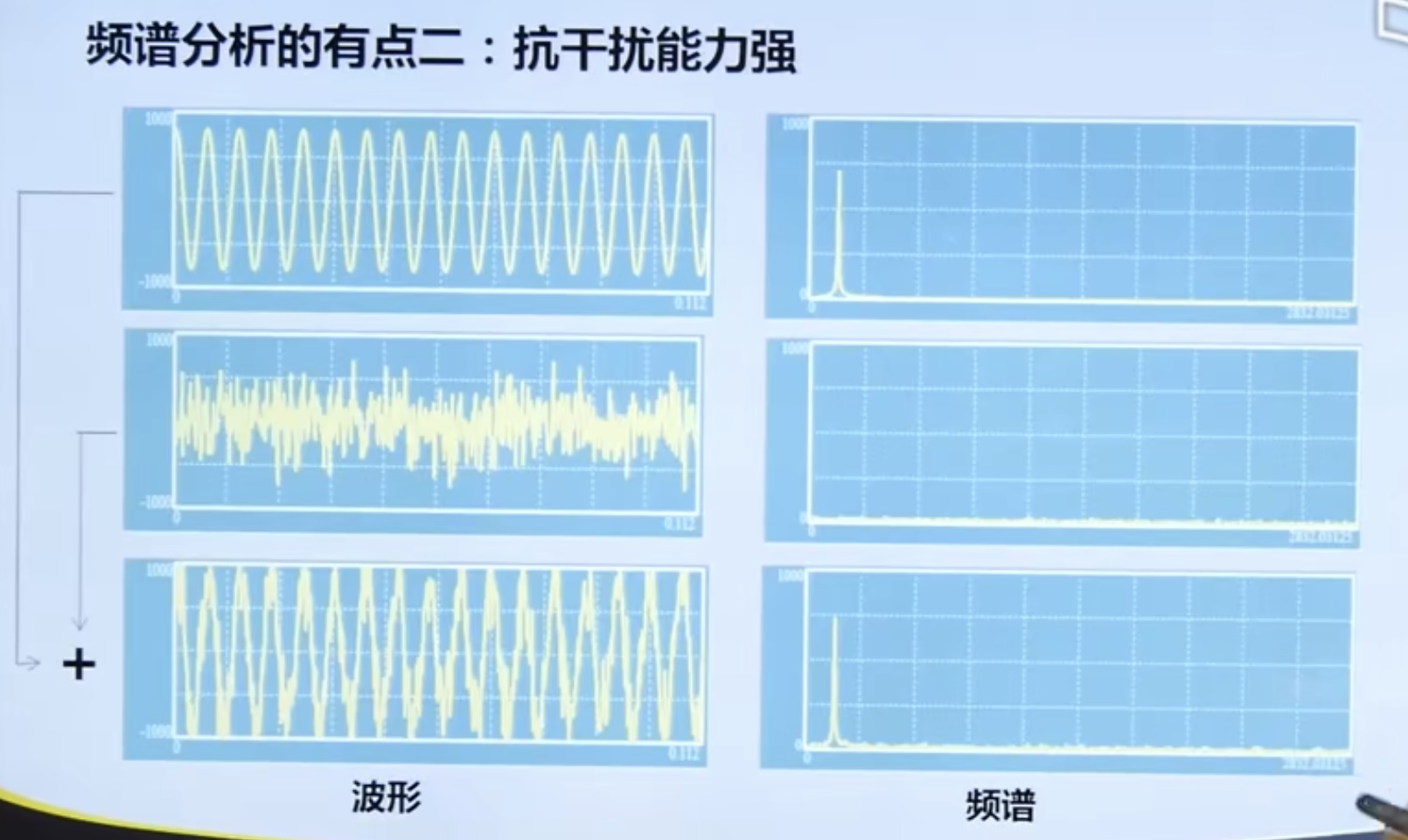
4.1. 2 advantages of spectrum analysis

1. It is convenient to analyze complex signals
2. Strong anti-interference ability
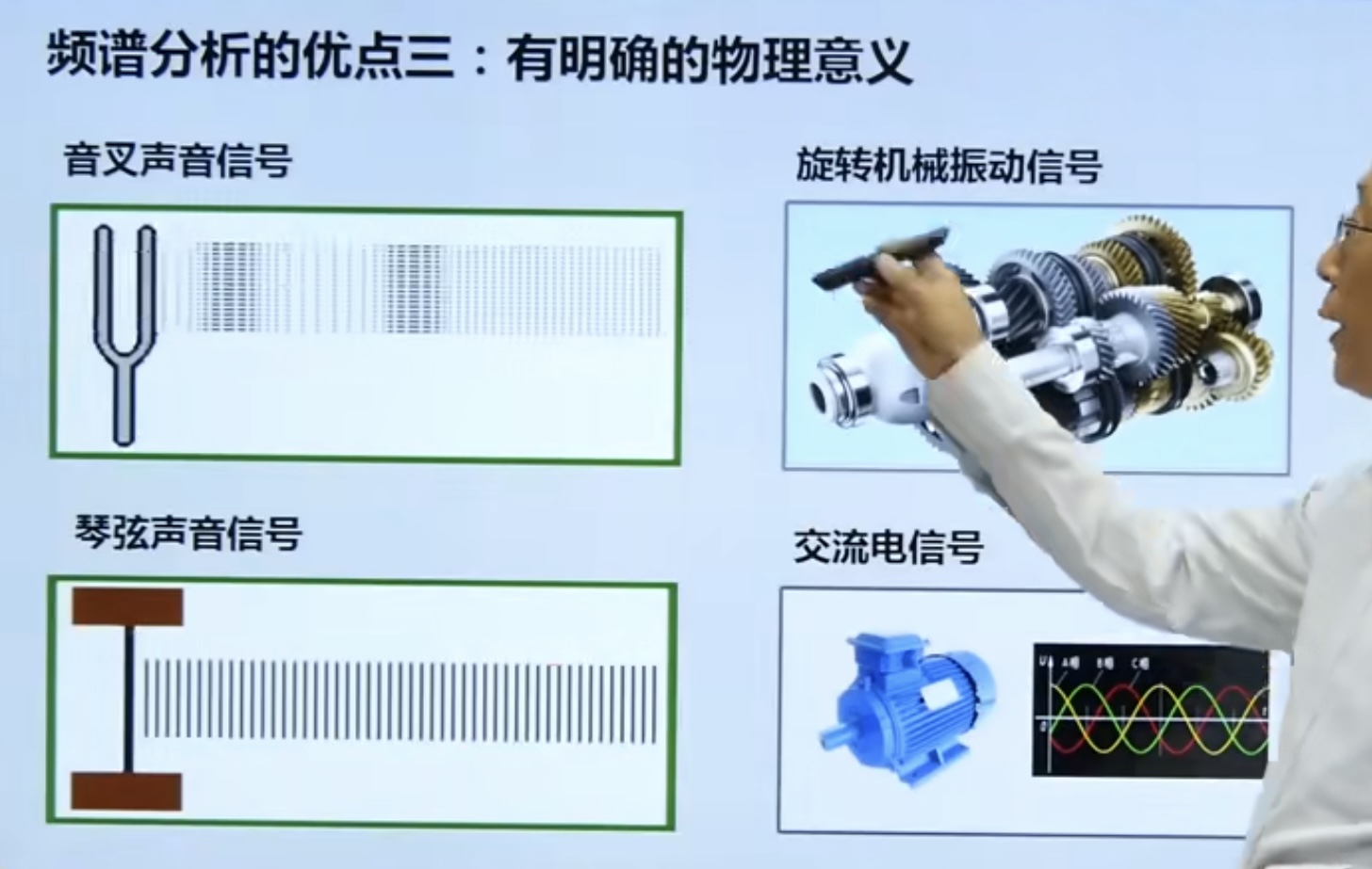
3. It has clear physical meaning

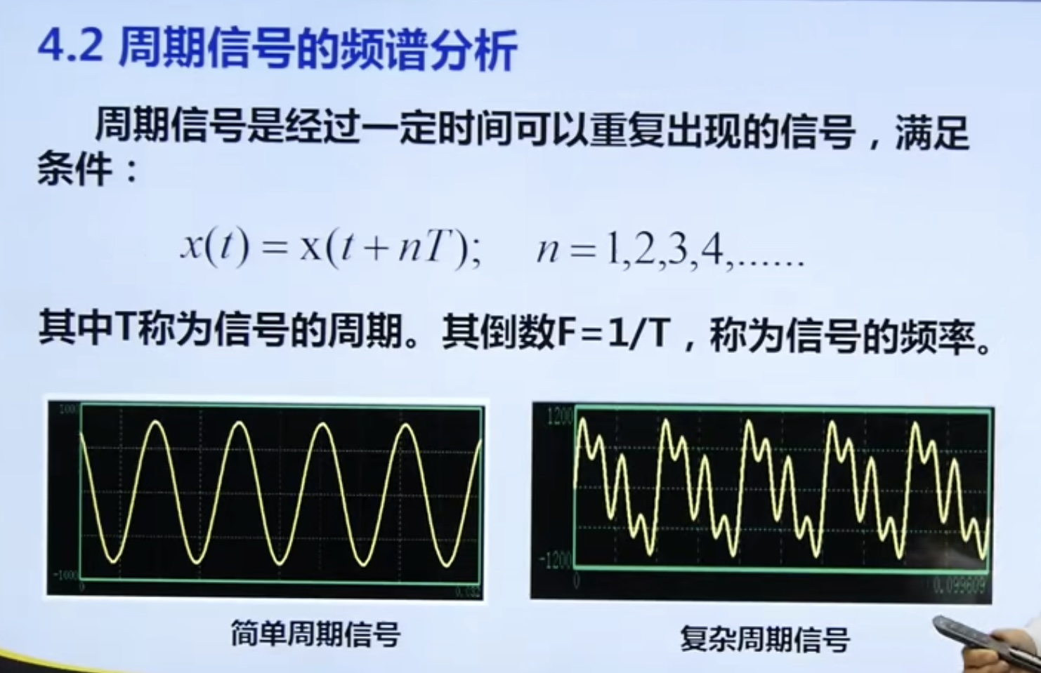
4.2 periodic signal spectrum analysis

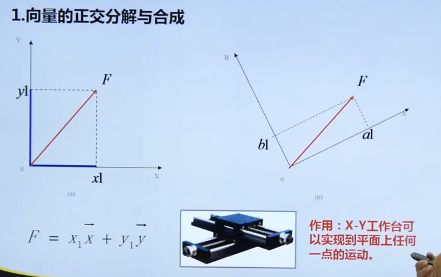
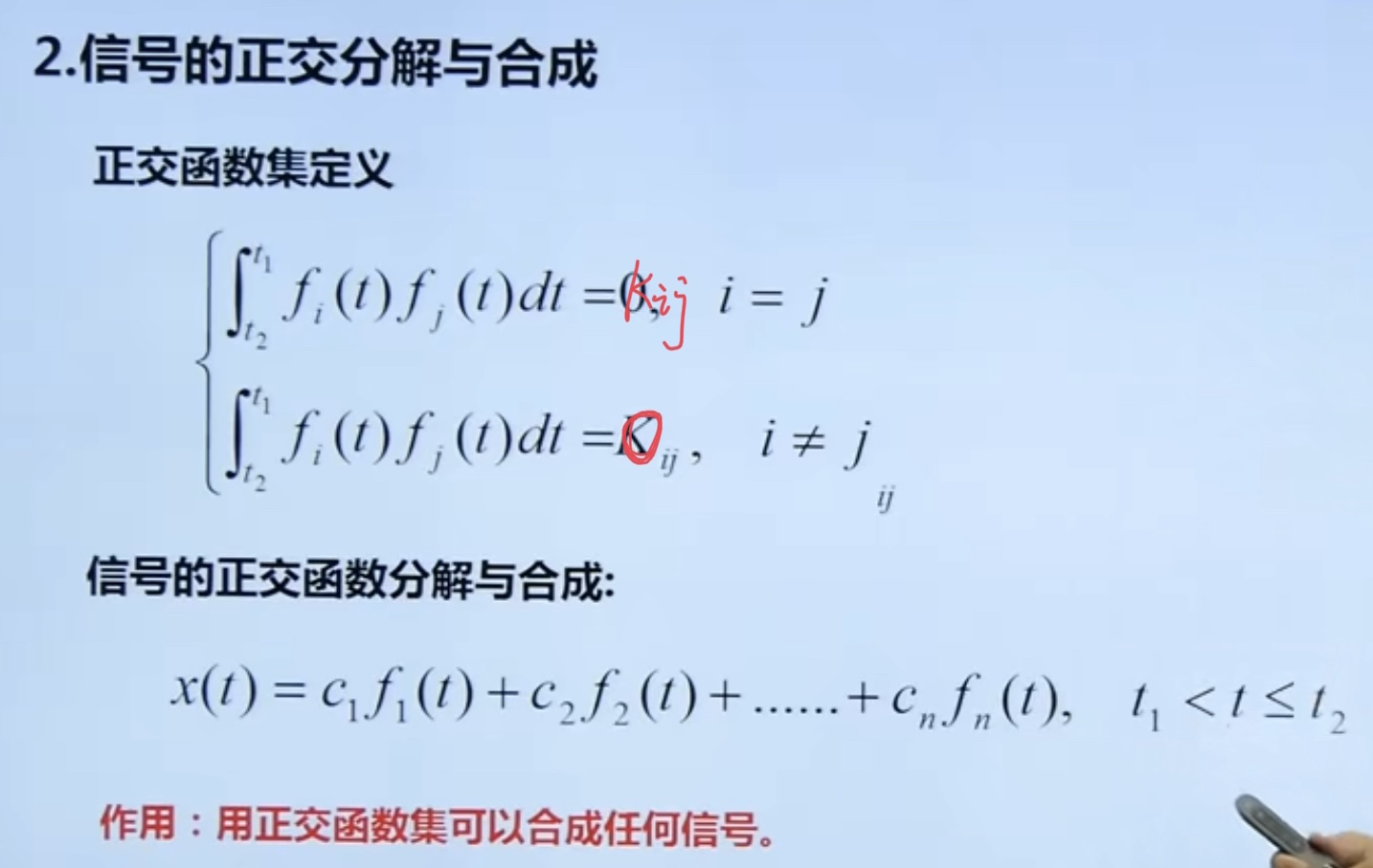
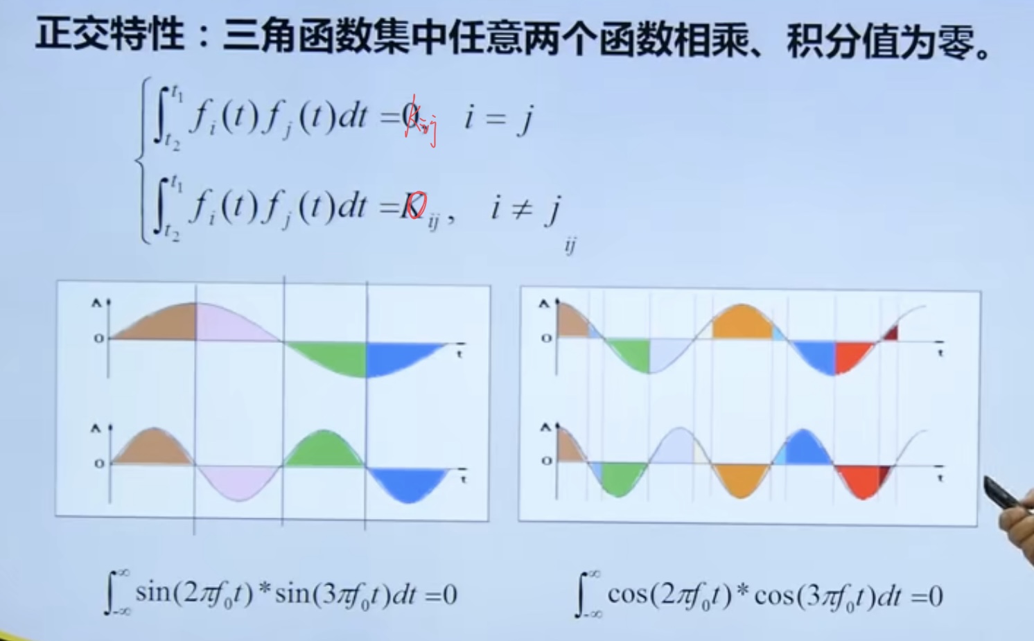
4.2. 1 Orthogonal Decomposition and synthesis

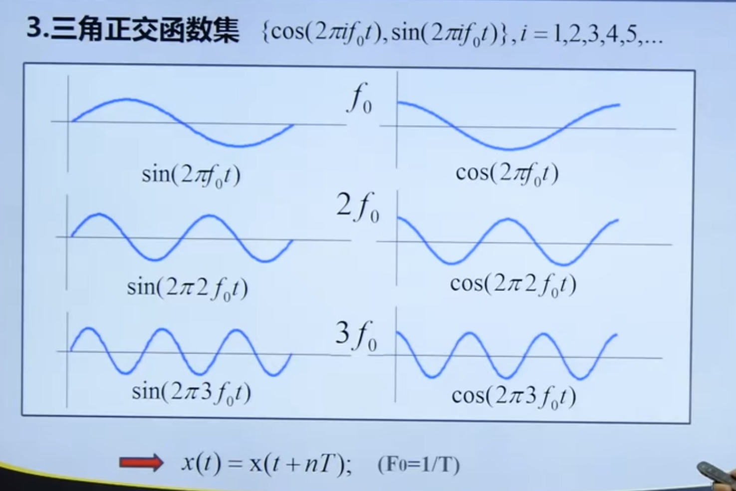
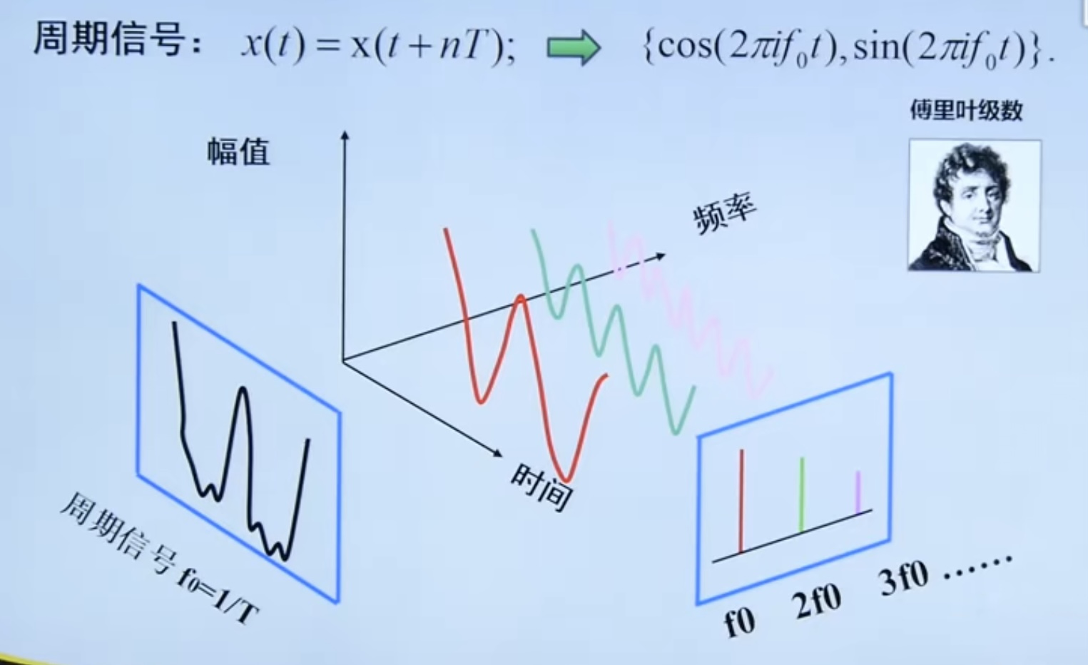
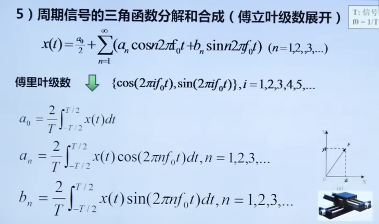
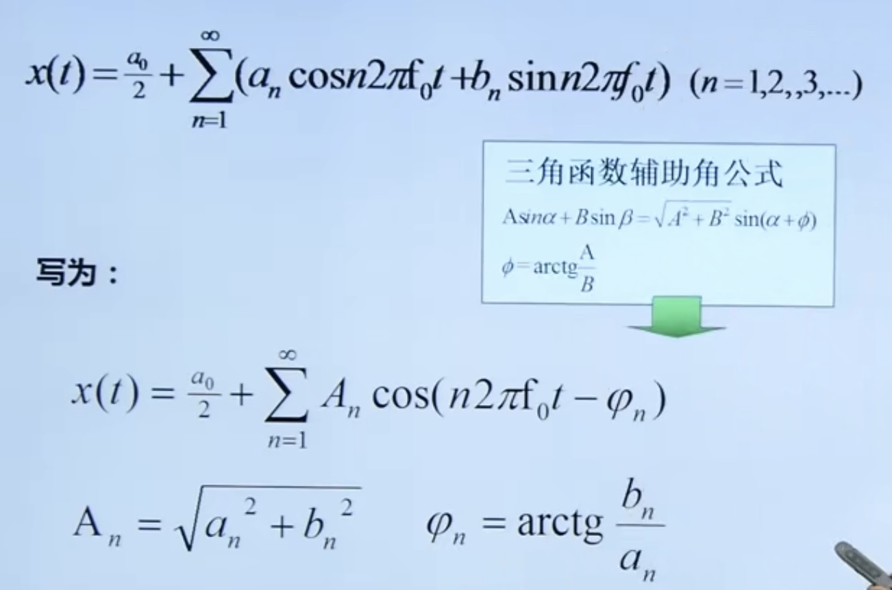
The periodic signal can be expressed by trigonometric transaction function



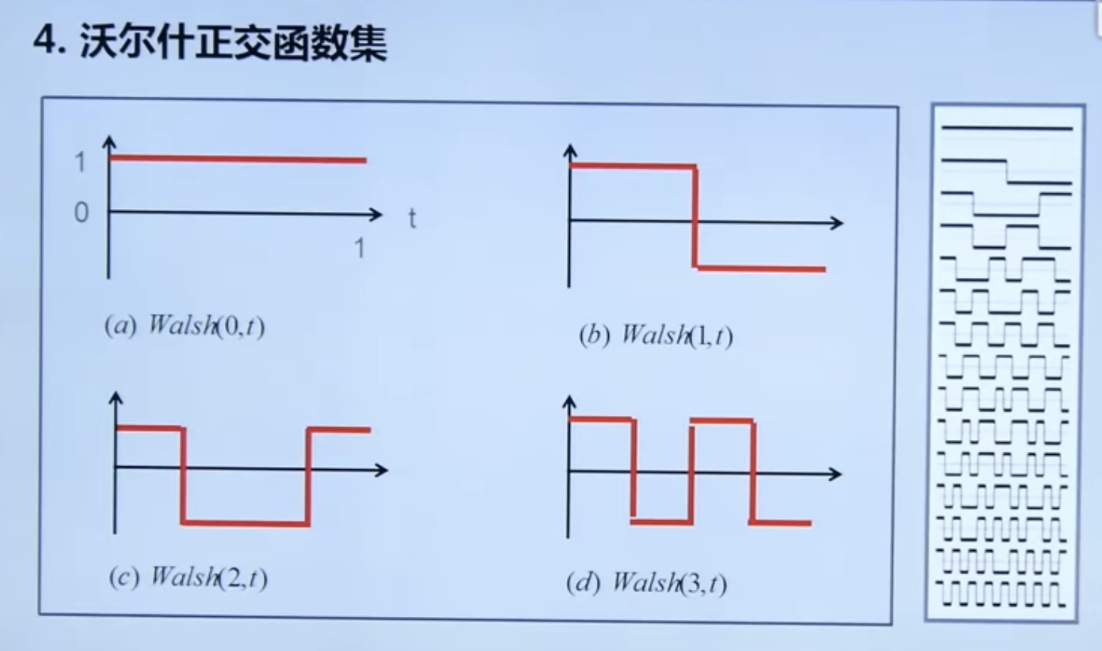
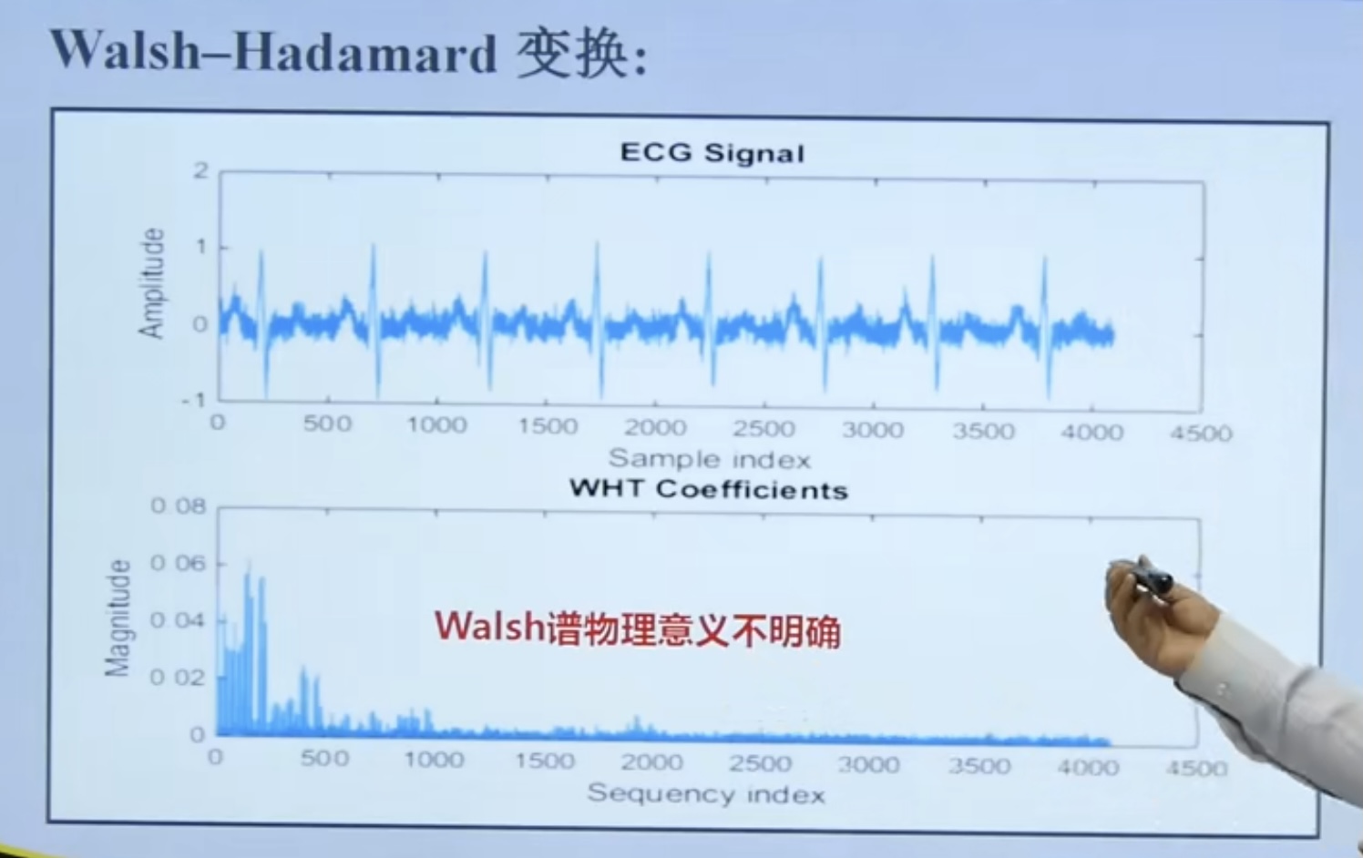
Because the spectrum physical meaning of Walsh orthogonal function set is not clear, it is less used.

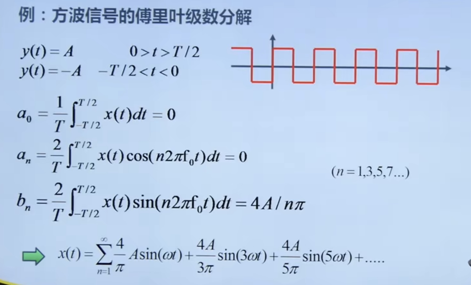
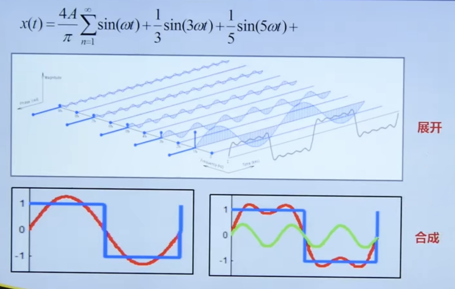
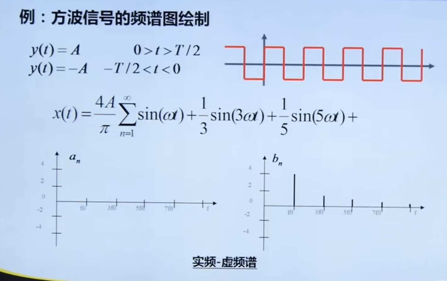
4.2. Triangular decomposition and synthesis of periodic signals

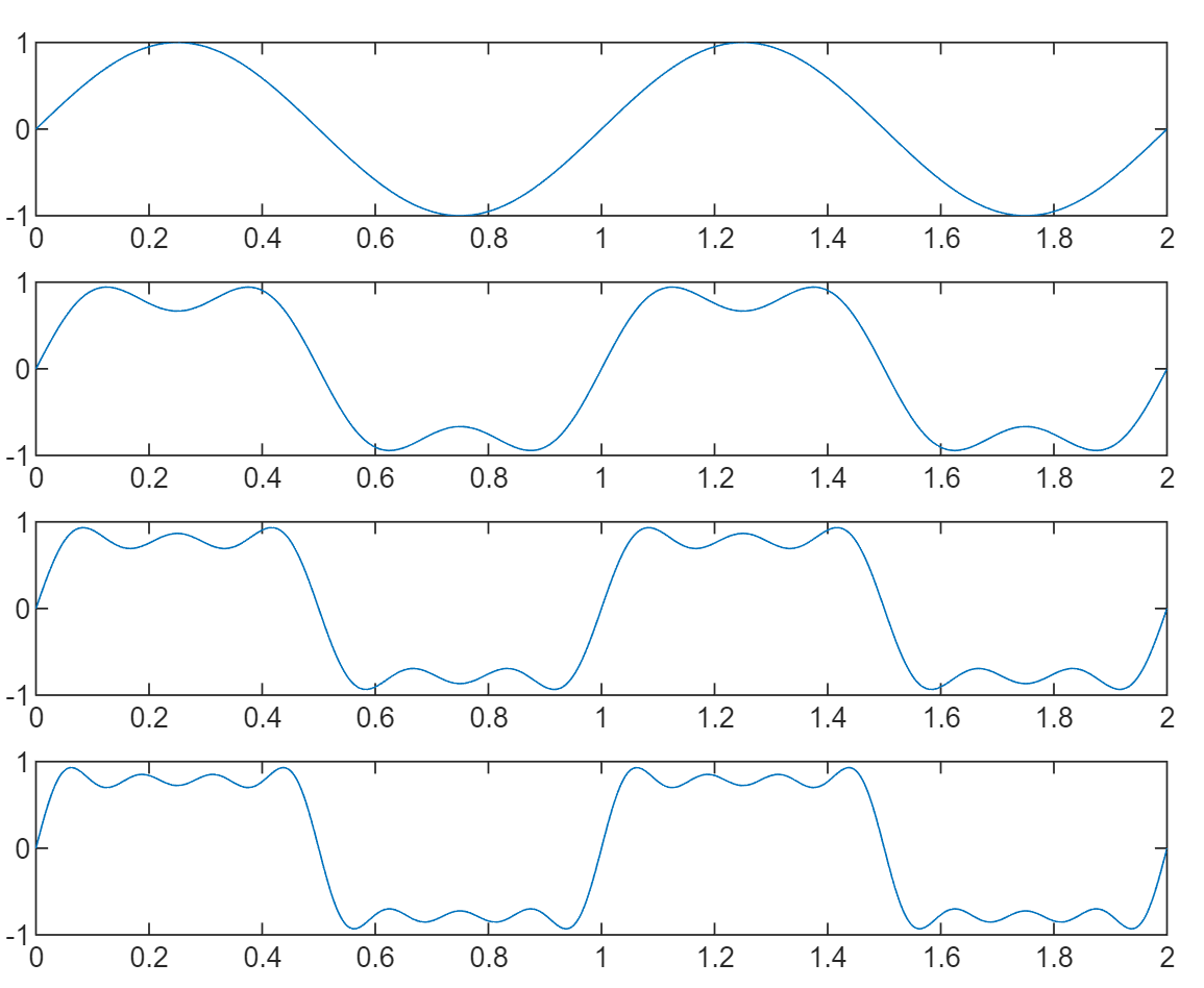
Decomposition and synthesis of square wave signal

MATLAB implementation

% Synthesis of square wave signal
N = 1024;T=2;
x = linspace(0,T,N);
y1 = sin(2*pi*x);
subplot(4,1,1)
plot(x,y1)
y2 = y1 + 1/3*sin(3*2*pi*x);
subplot(4,1,2)
plot(x,y2)
y3 = y2 + 1/5*sin(5*2*pi*x);
subplot(4,1,3)
plot(x,y3)
y4 = y3 + 1/7*sin(7*2*pi*x);
subplot(4,1,4)
plot(x,y4)

result:

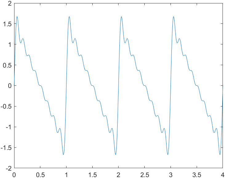
Decomposition and synthesis of sawtooth waves

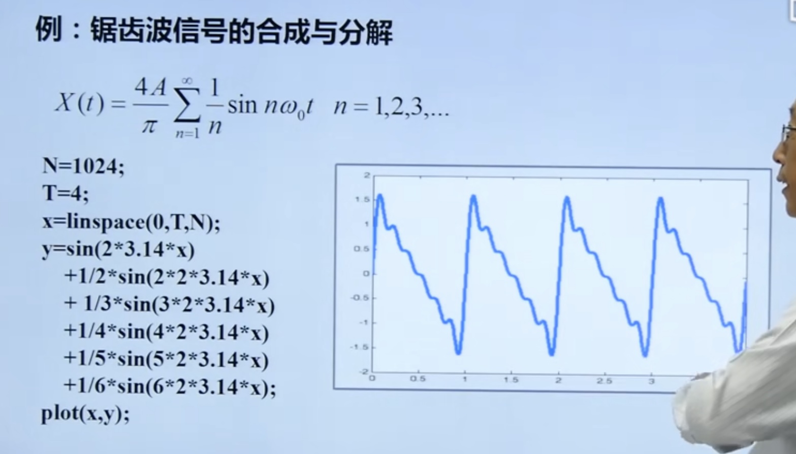
MATLAB implementation

% Synthesis of sawtooth signal
N = 1024;T=4;
x = linspace(0,T,N);
y = sin(2*pi*x)...
    + 1/2*sin(2*2*pi*x)...
    + 1/3*sin(3*2*pi*x)...
    + 1/4*sin(4*2*pi*x)...
    + 1/5*sin(5*2*pi*x)...
    + 1/6*sin(6*2*pi*x)...
    + 1/7*sin(7*2*pi*x)...
    + 1/8*sin(8*2*pi*x);
figure
plot(x,y)

result:

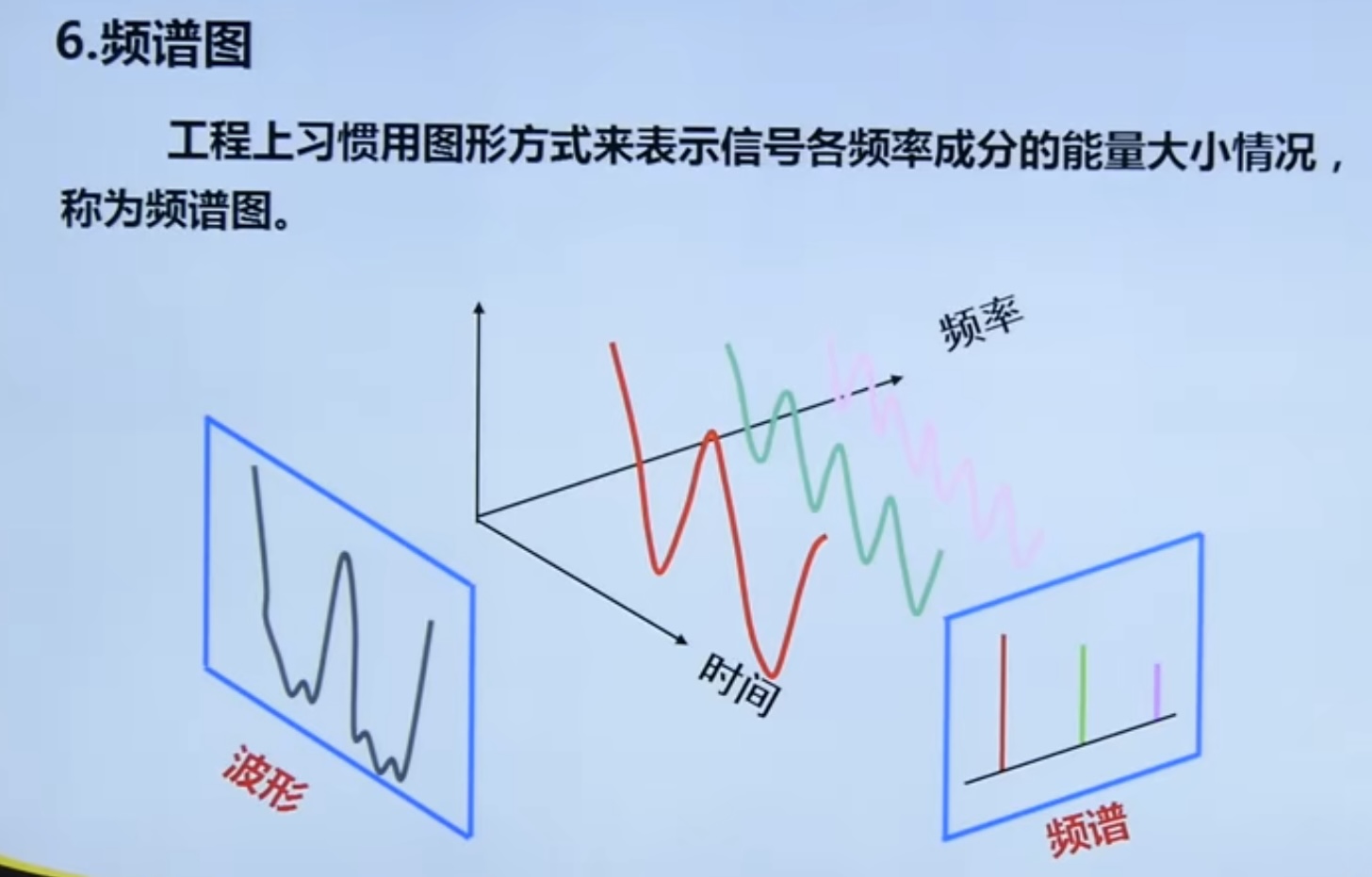
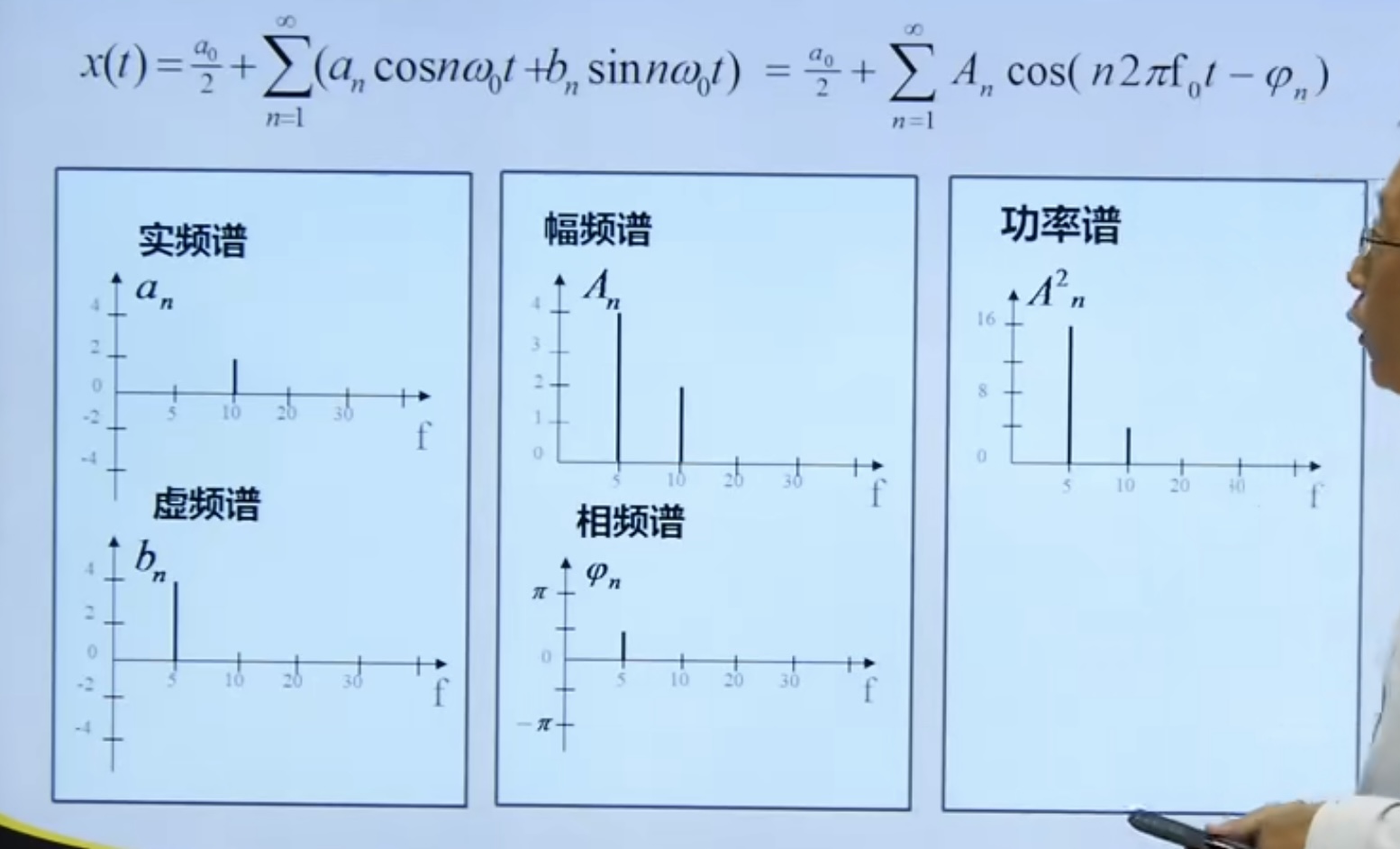
4.2. 3 spectrum diagram

Logarithmic power spectrum

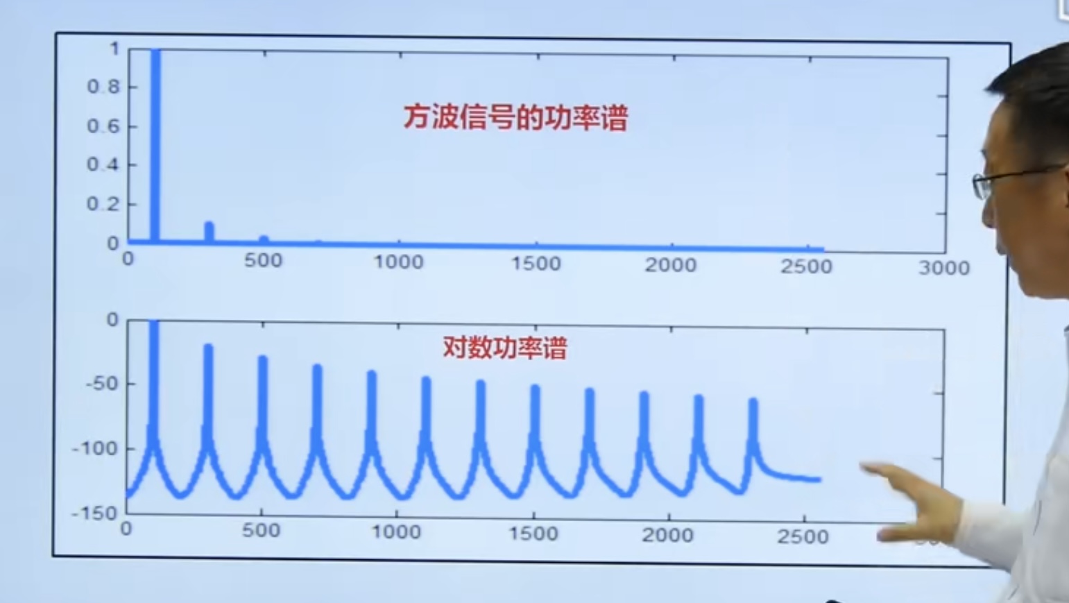
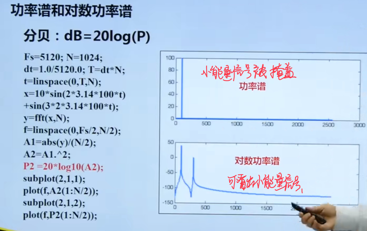
Logarithmic power spectrum can show the power of small signal.

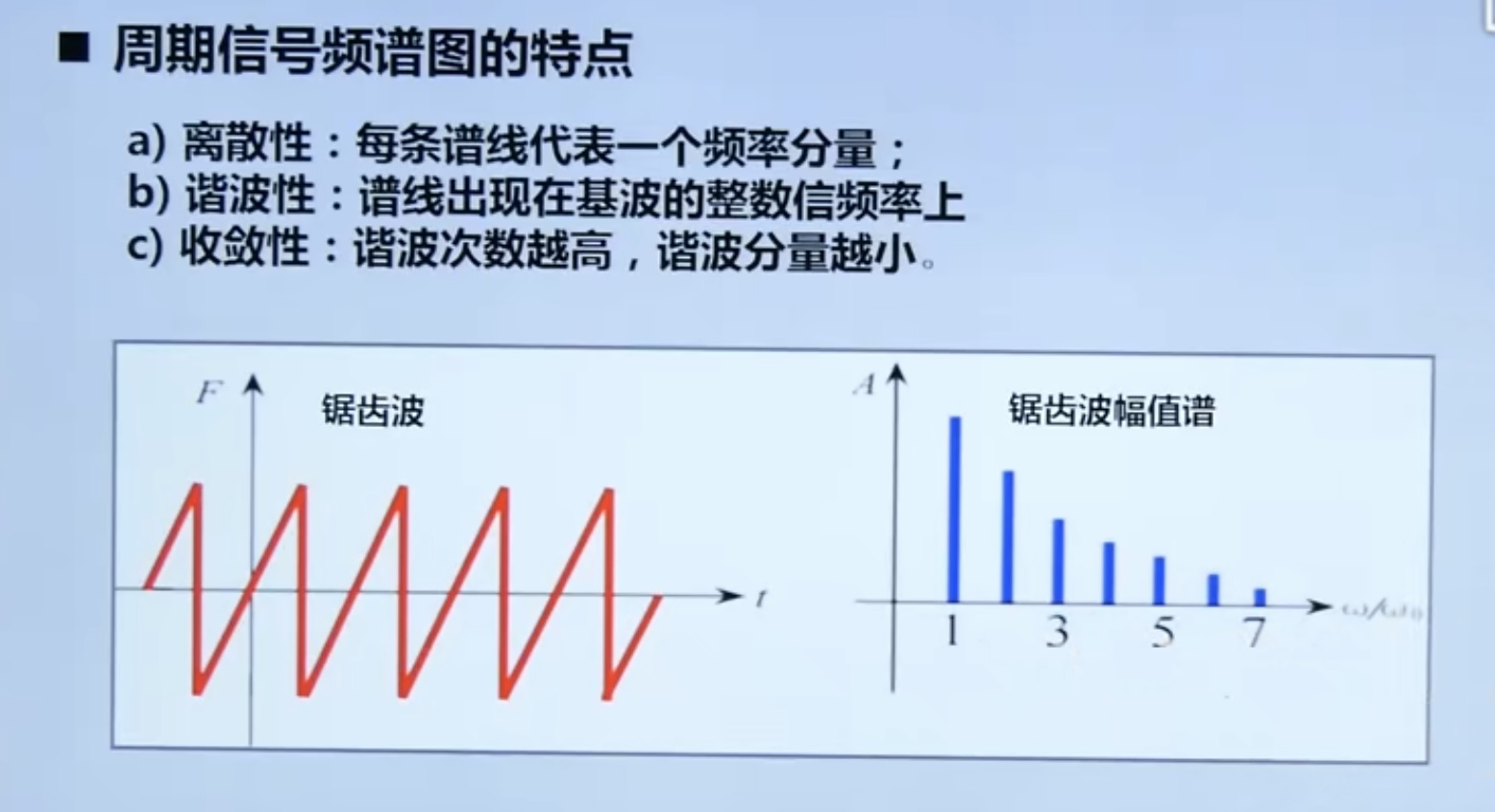
Characteristics of periodic signal spectrum

1. Discreteness; 2. Harmonics; 3. Convergence

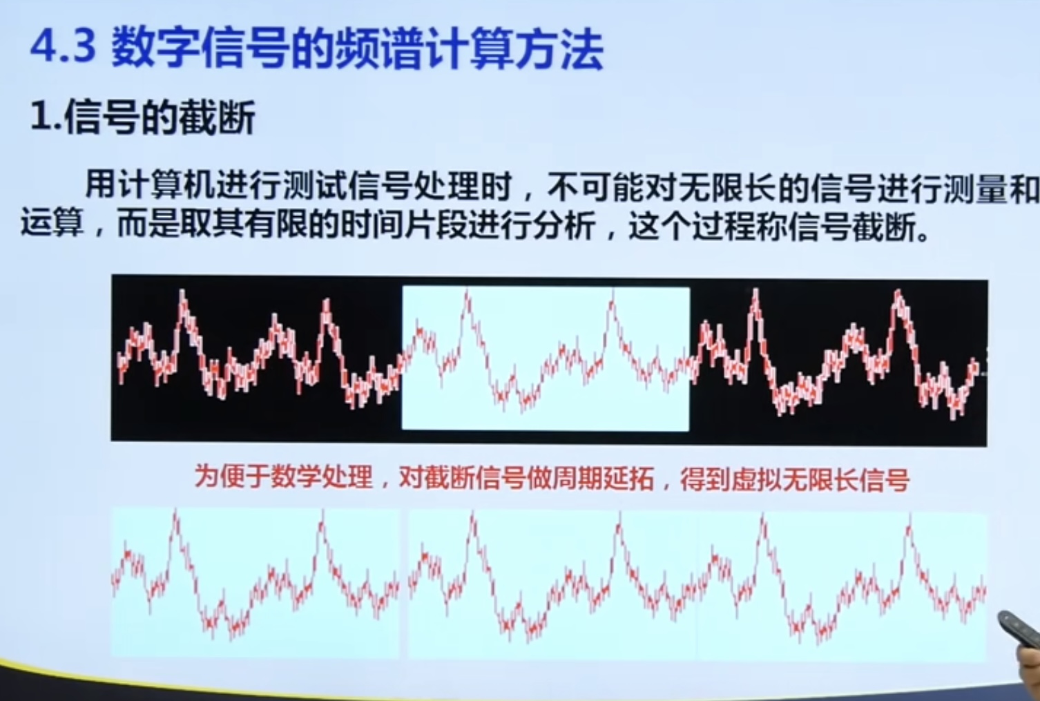
4.3 calculation method of digital signal spectrum

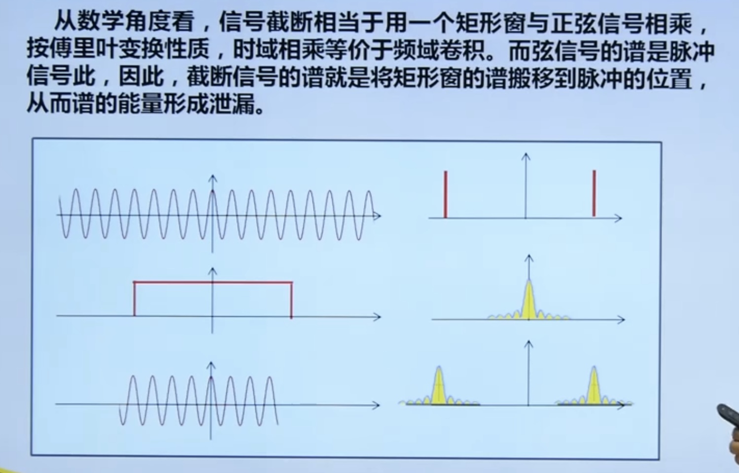
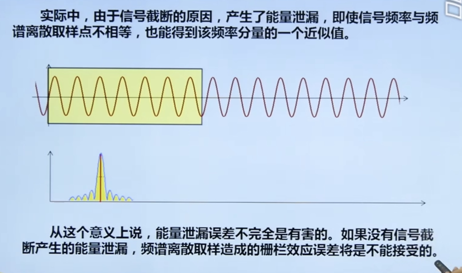
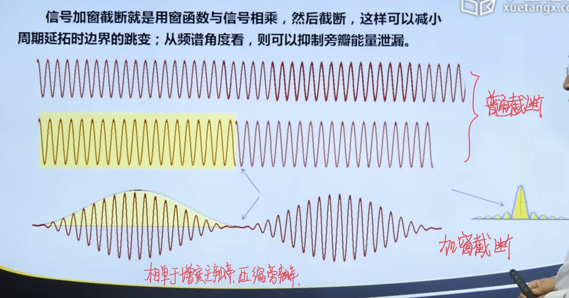
4.3. 1 signal truncation and energy leakage

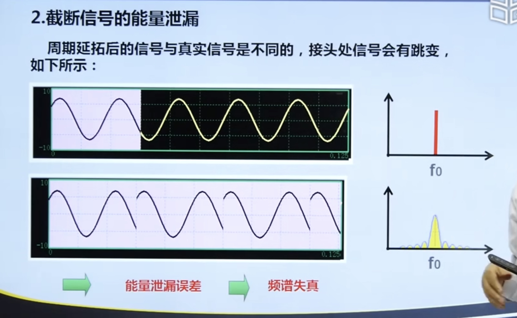
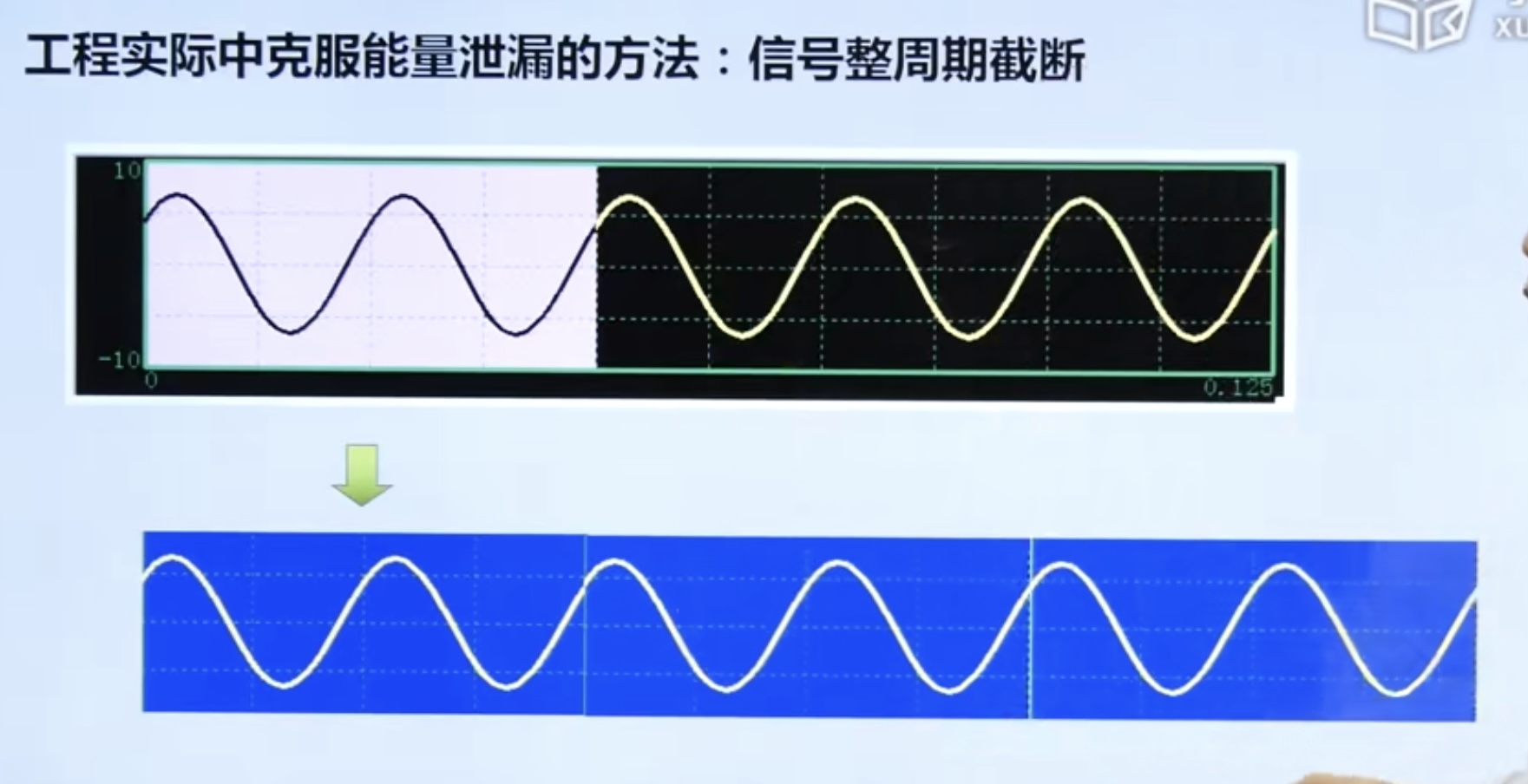
Ways to overcome energy leakage

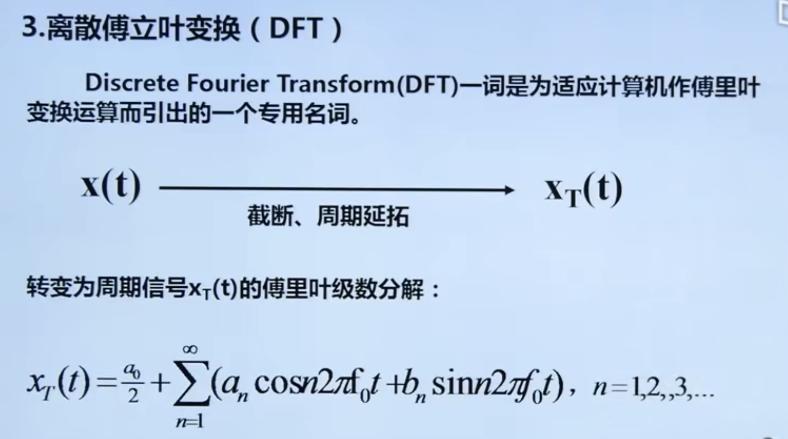
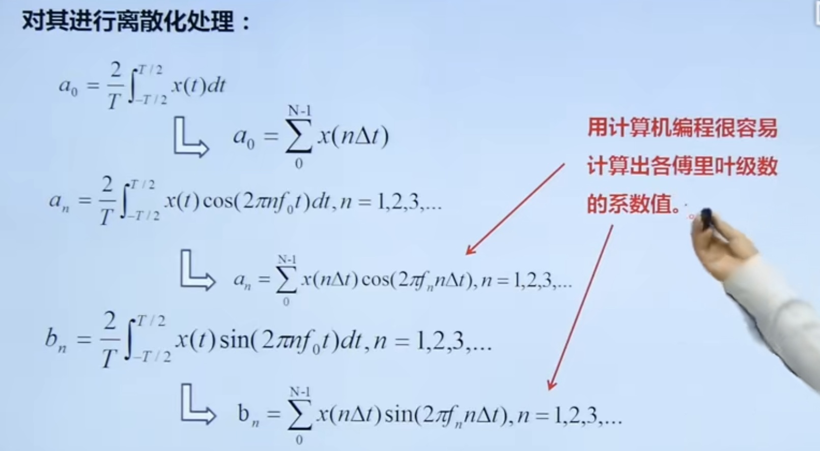
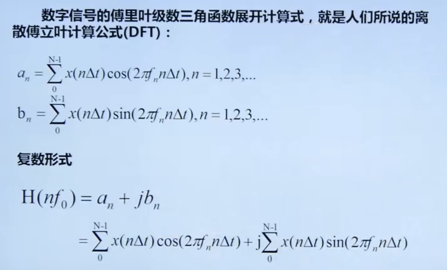
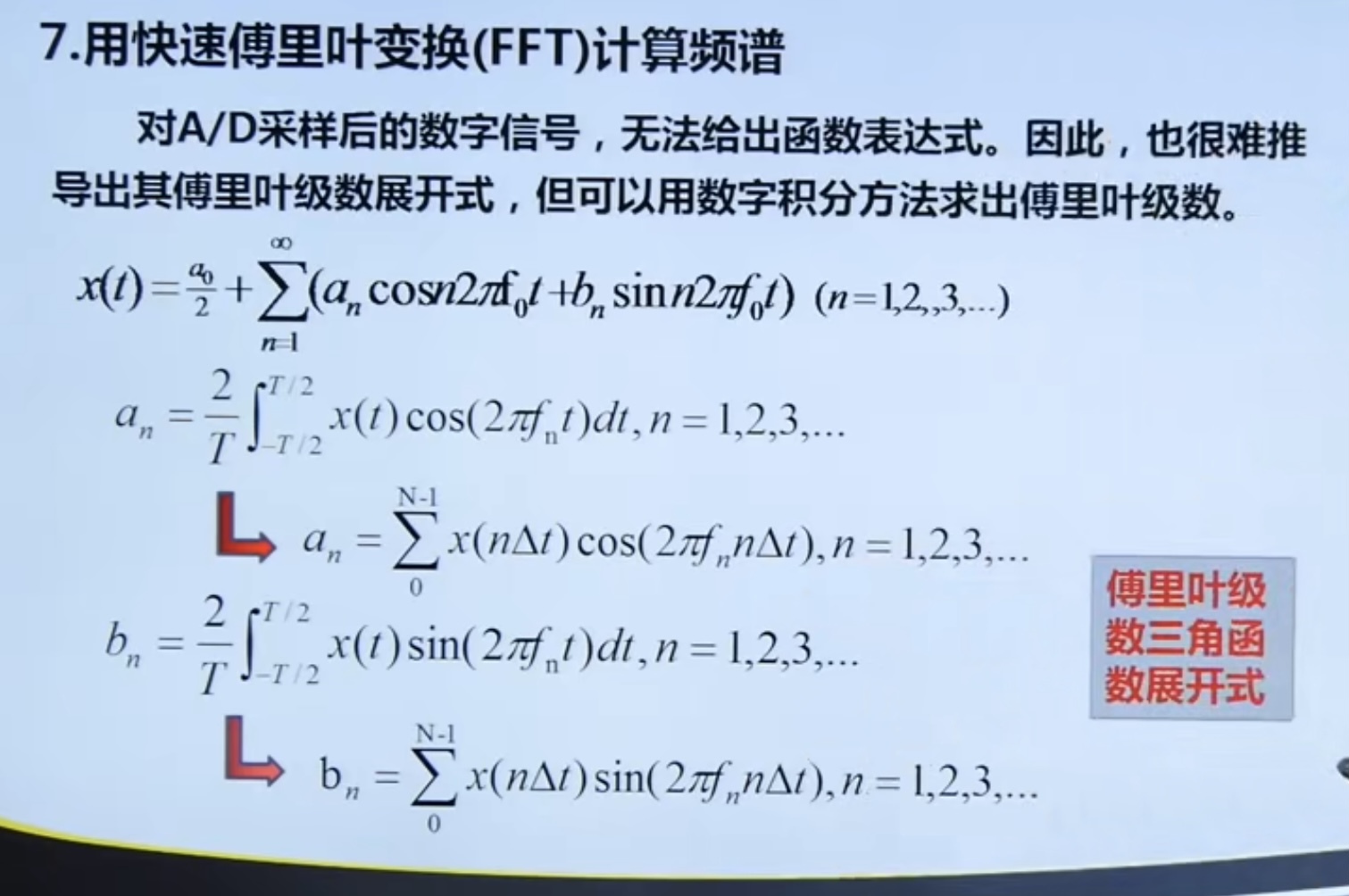
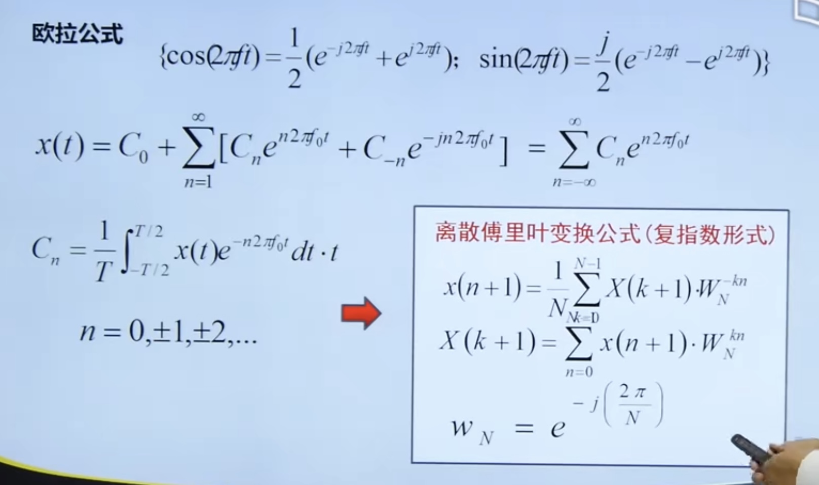
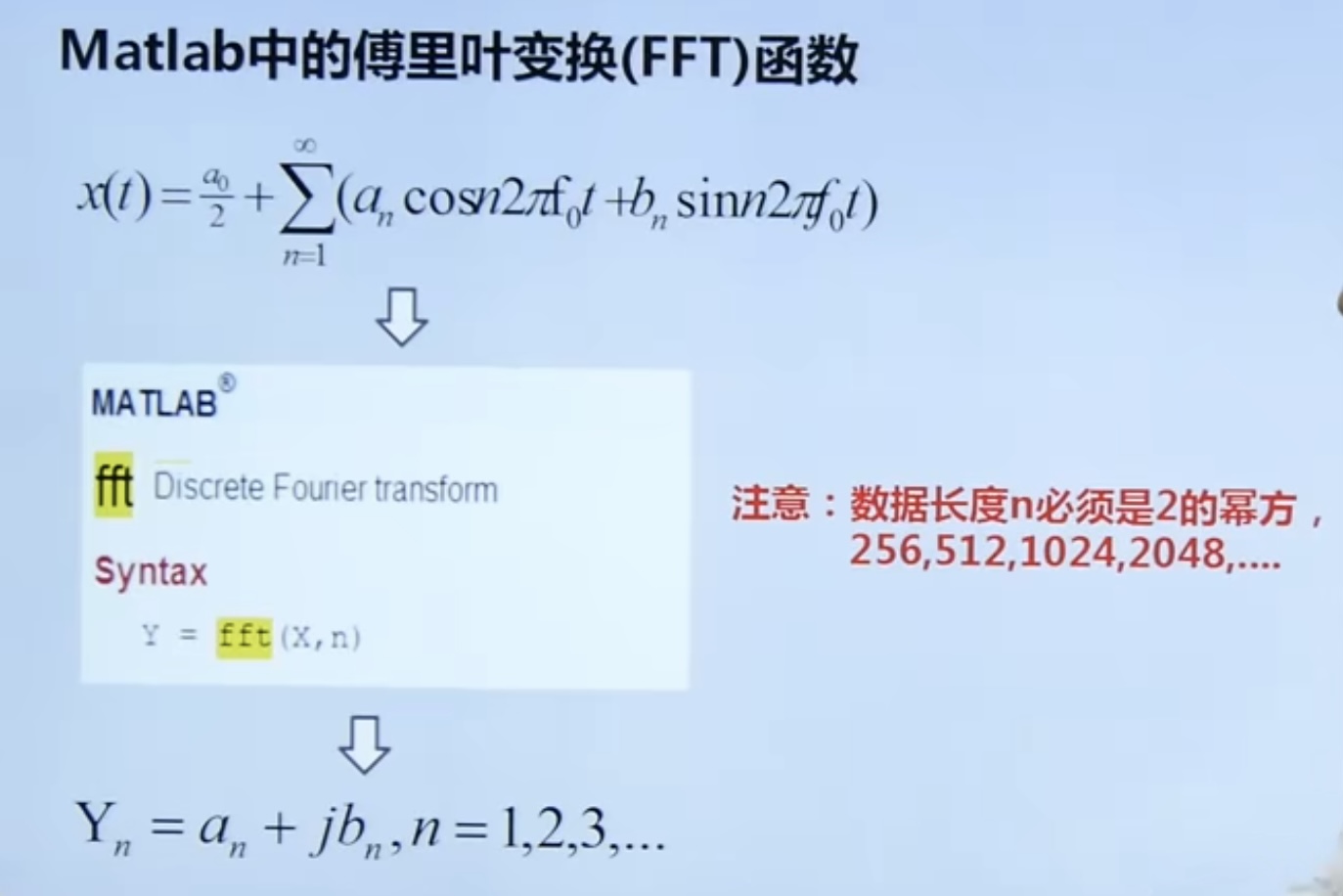
4.3. 2 discrete Fourier transform (DFT)

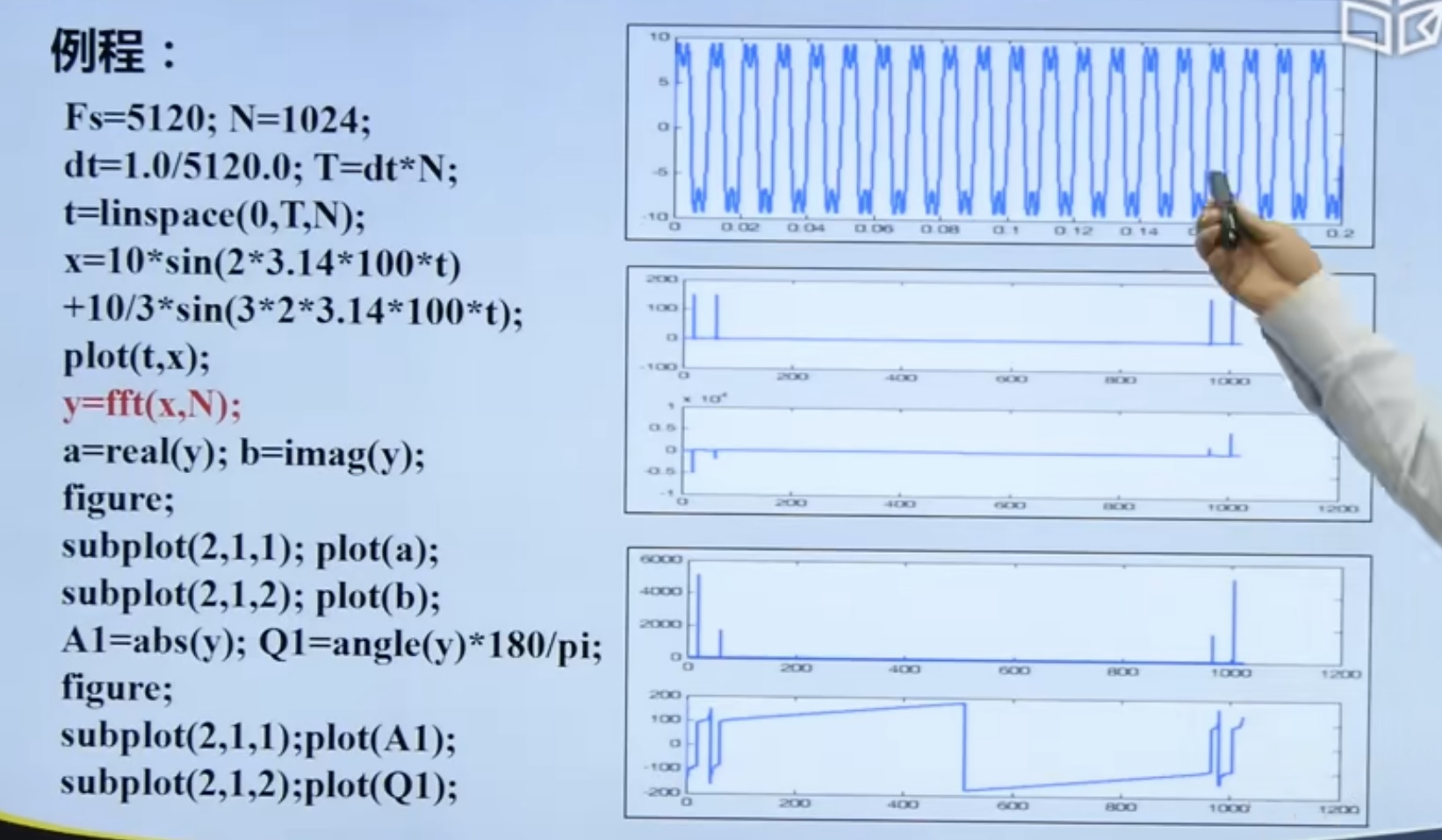
4.3. 3 fast Fourier transform (FFT)

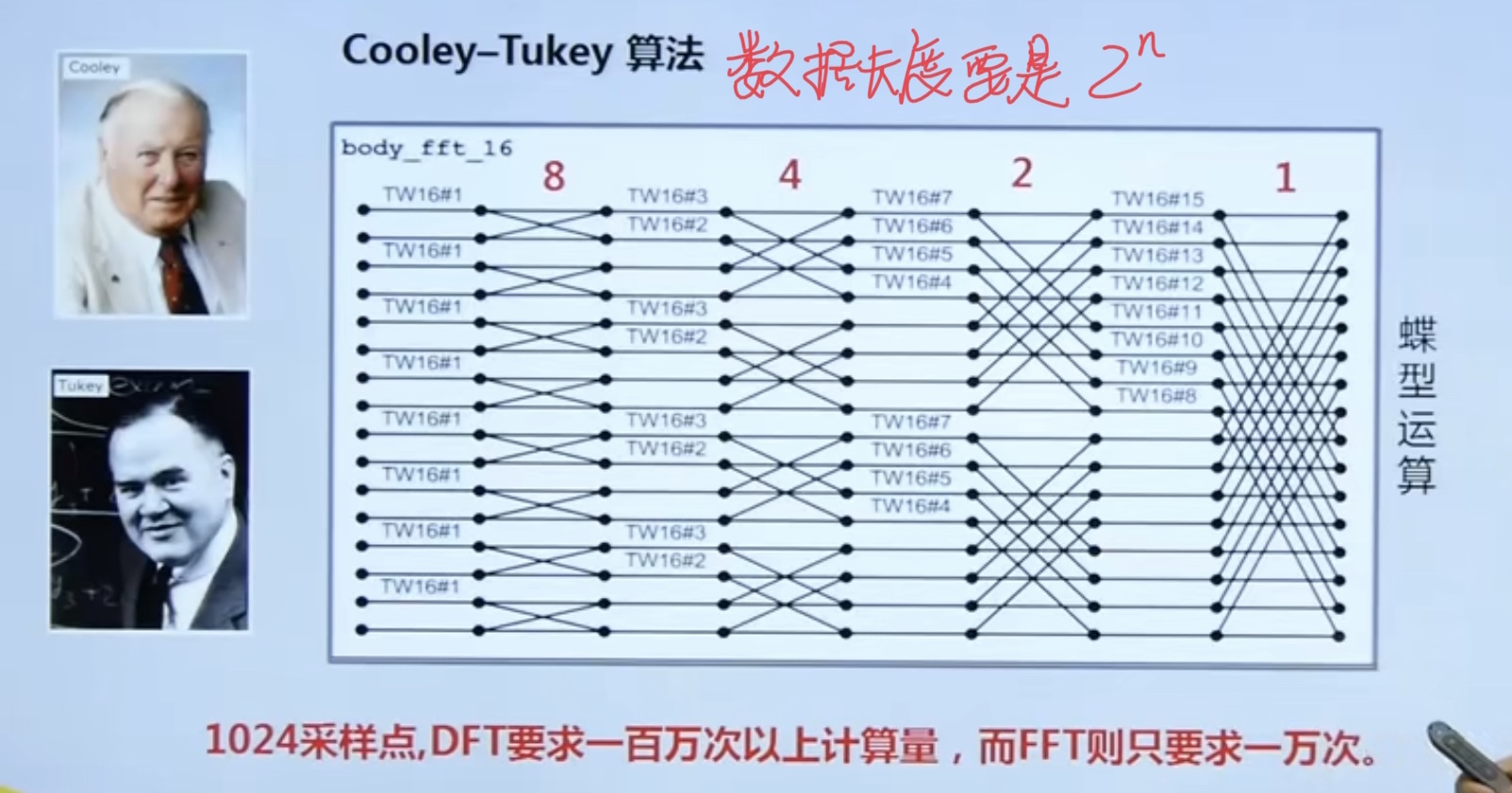
FFT greatly reduces the computational complexity of DFT and makes the calculation faster.

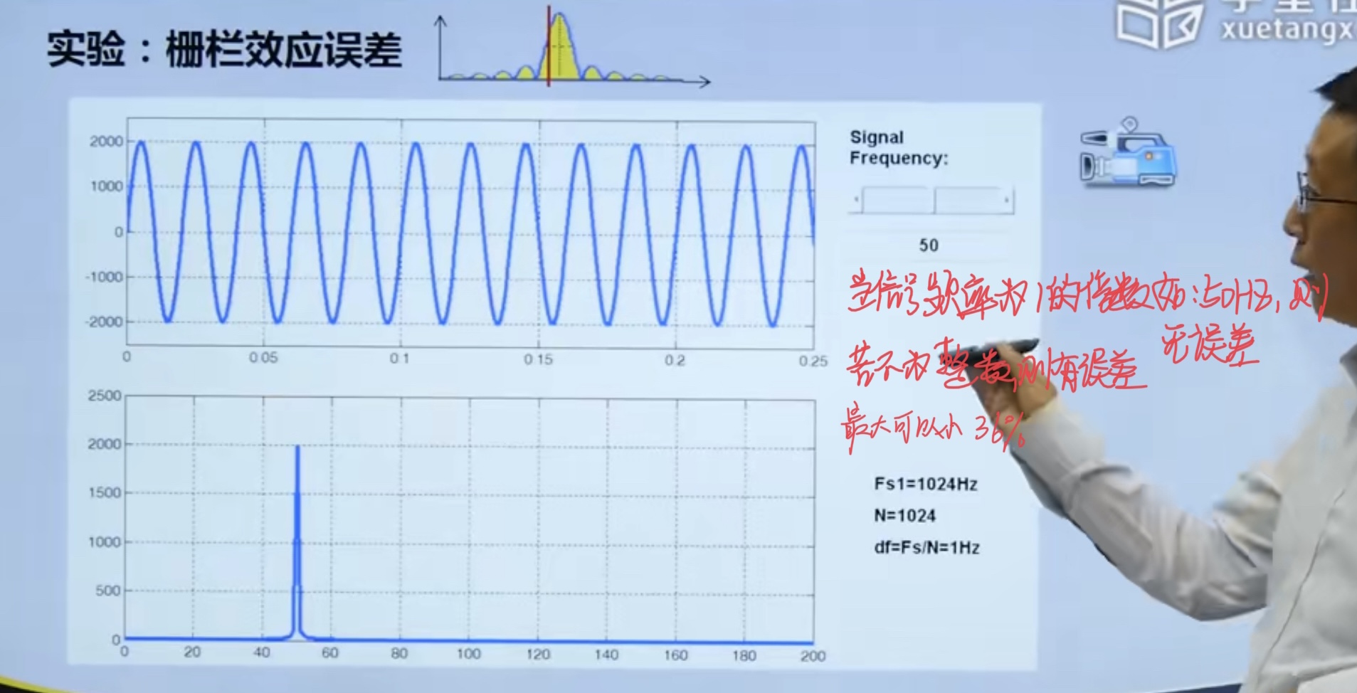
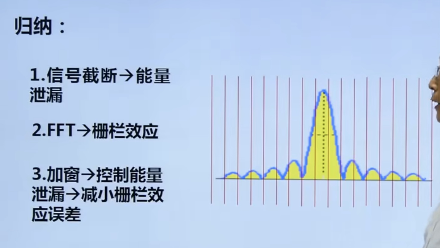
4.4 fence effect

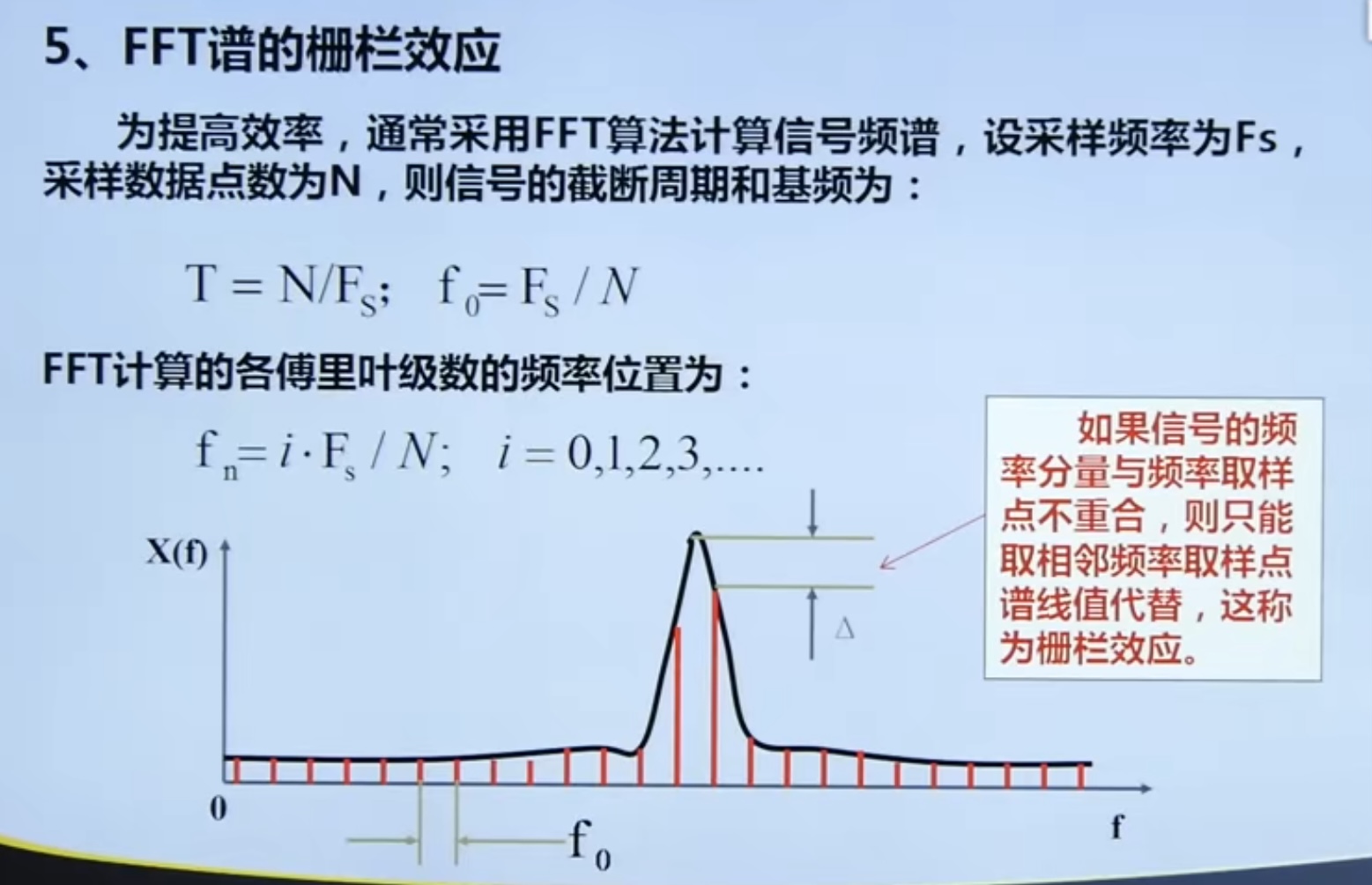
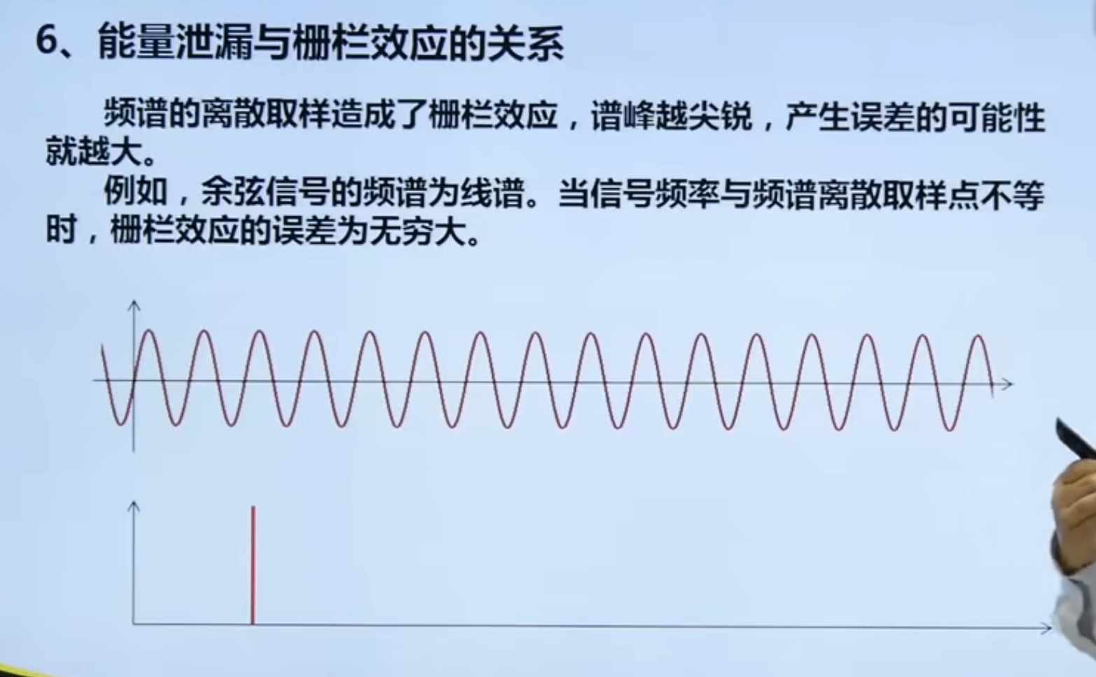
4.4. 1 Relationship between energy leakage and fence effect

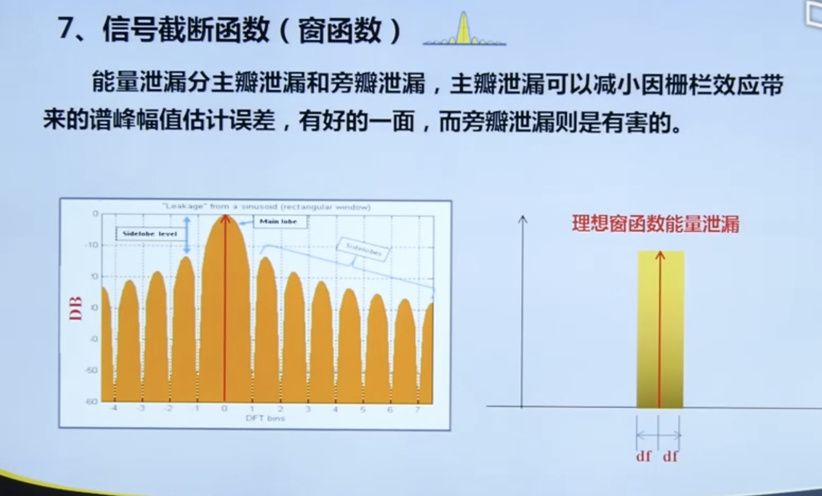
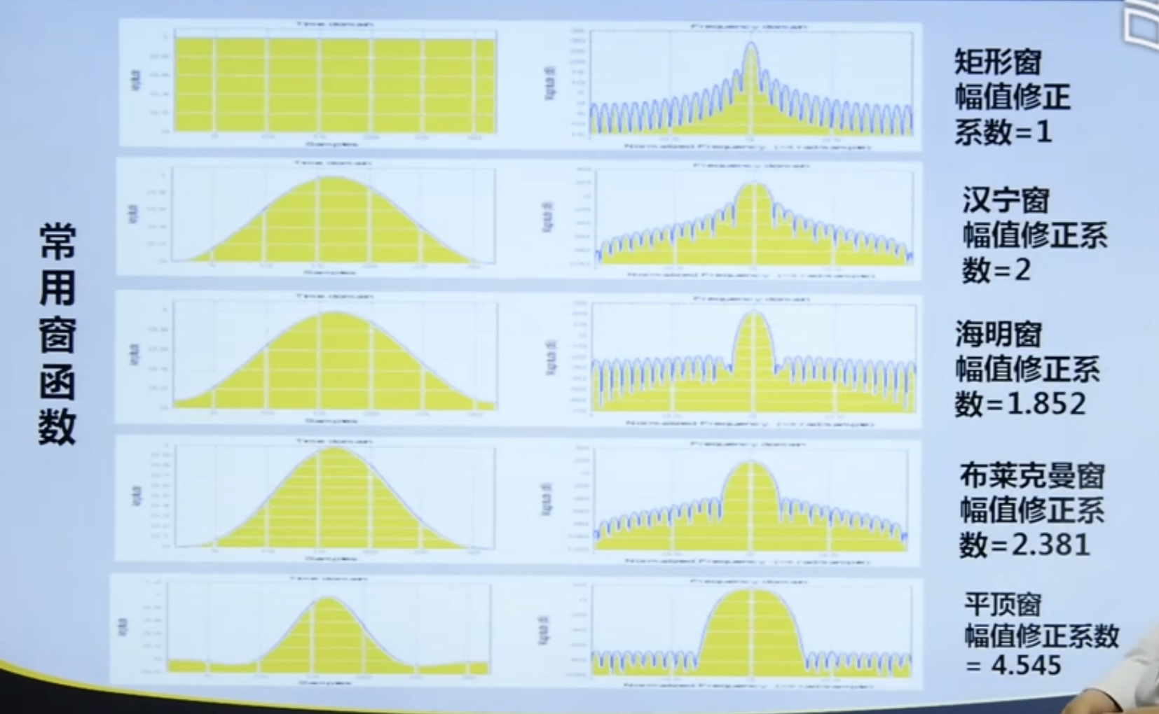
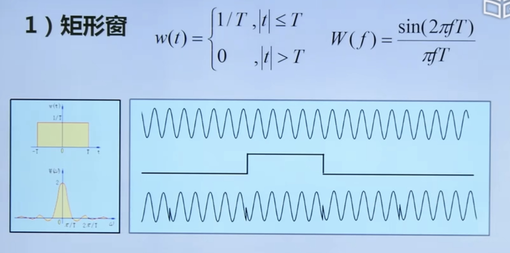
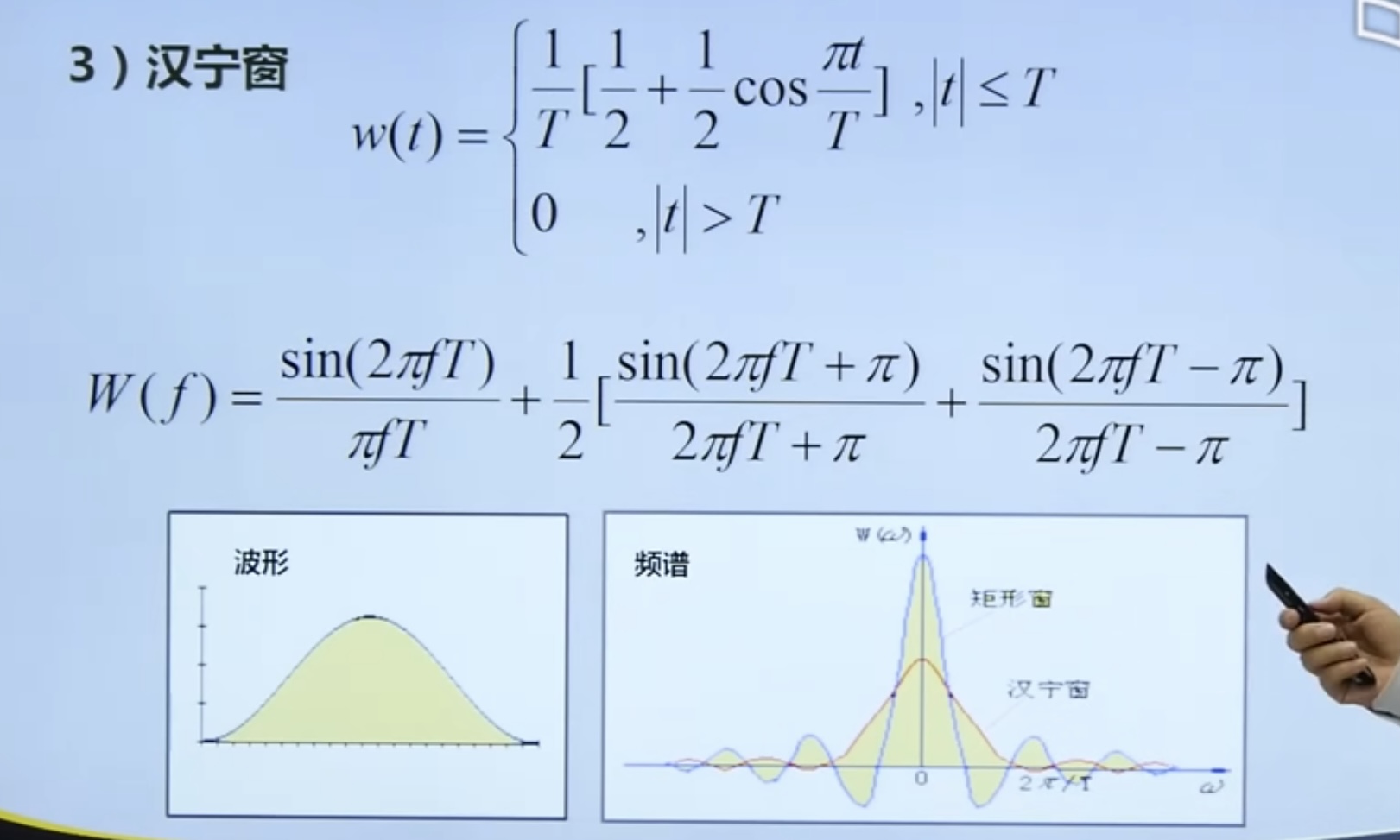
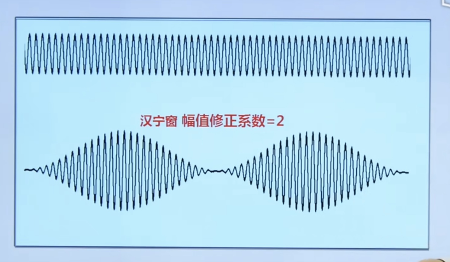
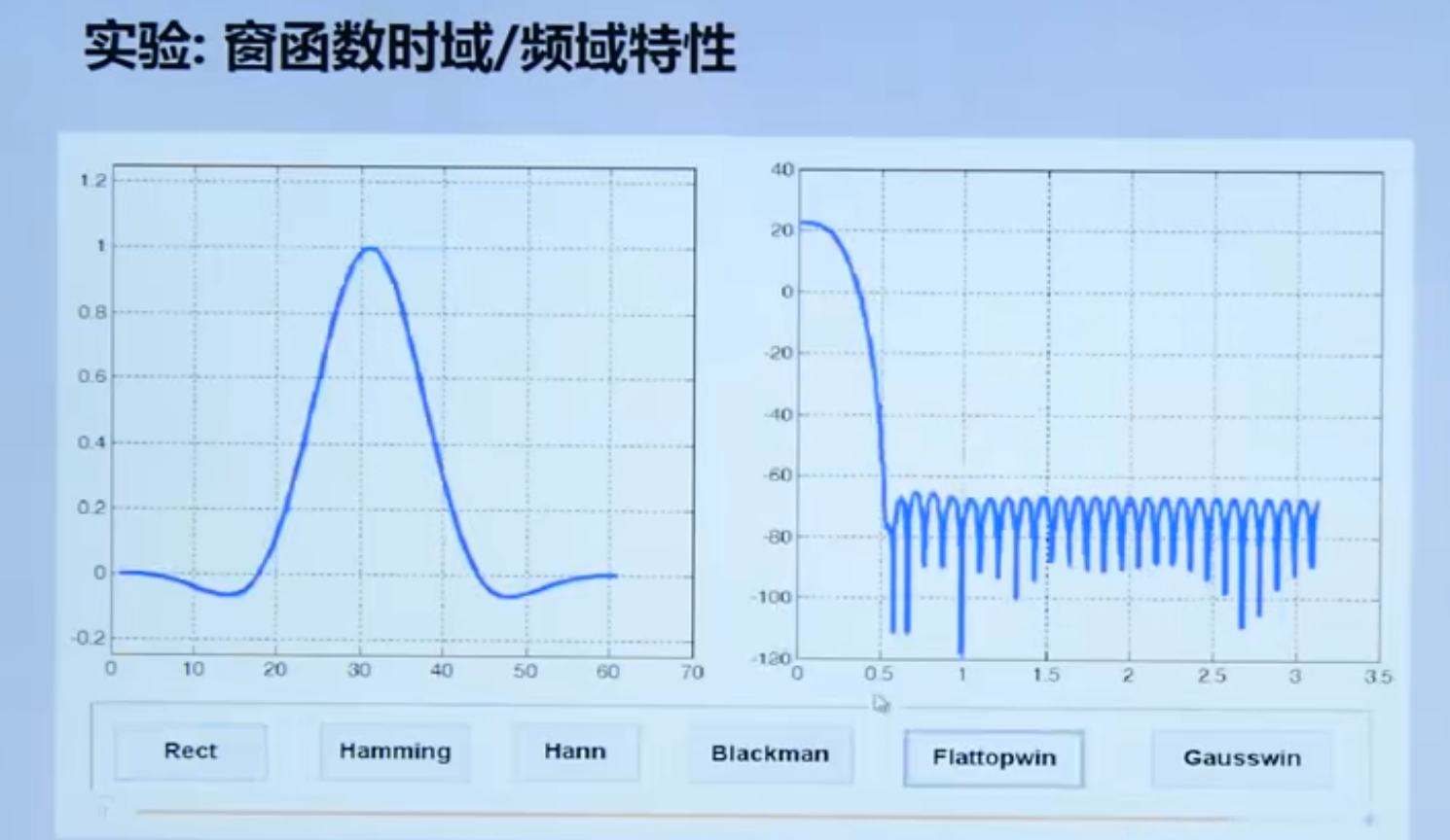
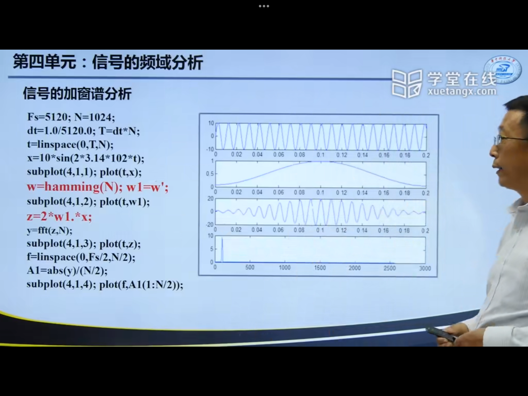
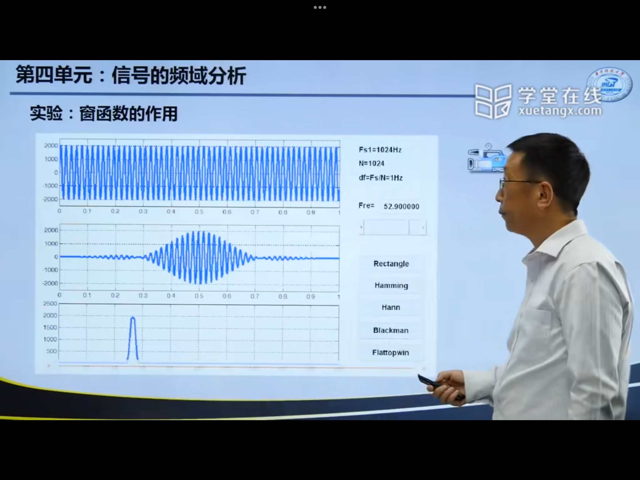
4.4. 2 windowed function

Common window functions

4.4. 3 Summary

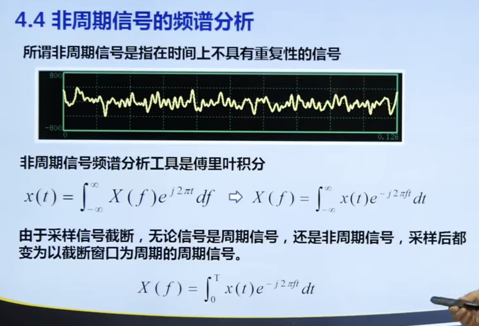
4.4 spectrum analysis of aperiodic signal

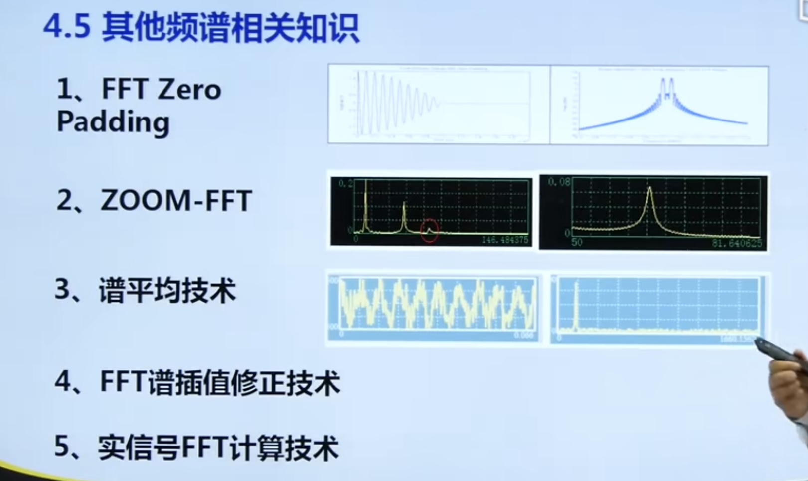
4.5 other spectrum related knowledge

Spectrum analysis is mainly used to identify the periodic component in the signal. It is the most commonly used means in signal analysis.

Job:

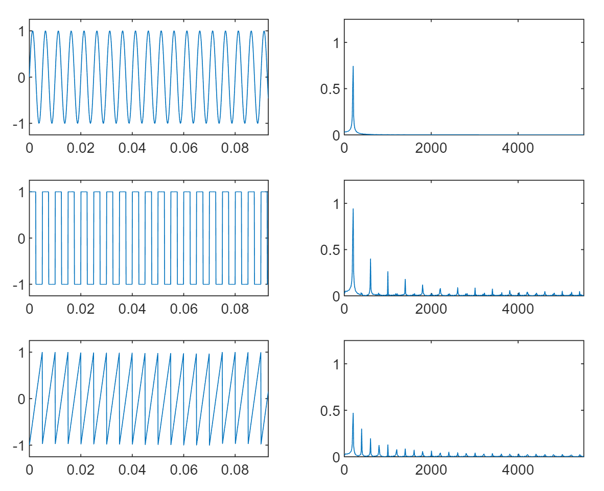
1. The sine wave, square wave and triangular wave with amplitude of 10 and frequency of 200Hz are sampled and transformed by 1024 point FFT at the sampling rate of 11025Hz, and their signal waveform and amplitude spectrum are drawn.

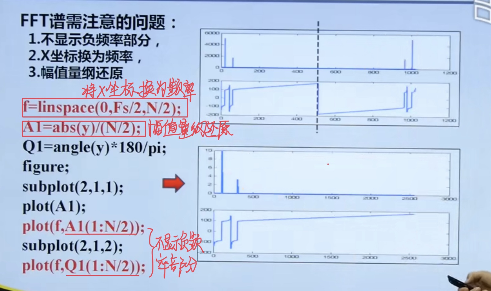
Fs = 11025;         % Adopted frequency
F = 200;            % signal frequency 
N = 1024;           % Sampling points
dt = 1/Fs;          % Sampling interval
T = dt*N;           % Total sampling time
t = linspace(0,T,N);% Sampling time
x1 = sin(2*pi*F*t);
x2 = square(2*pi*F*t);
x3 = sawtooth(2*pi*F*t);
y1 = fft(x1,N);
y2 = fft(x2,N);
y3 = fft(x3,N);
f = linspace(0,Fs/2,N/2);% x Coordinate conversion to frequency
figure
subplot(3,2,1)
plot(t,x1)
axis([-inf,inf,-1.25,1.25]);
subplot(3,2,2)
plot(f,abs(y1(1:N/2))/(N/2))
axis([-inf,inf,0,1.25]);
subplot(3,2,3)
plot(t,x2)
axis([-inf,inf,-1.25,1.25]);
subplot(3,2,4)
plot(f,abs(y2(1:N/2))/(N/2))
axis([-inf,inf,0,1.25]);
subplot(3,2,5)
plot(t,x3)
axis([-inf inf -1.25 1.25])
subplot(3,2,6)
plot(f,abs(y3(1:N/2))/(N/2))
axis([-inf,inf,0,1.25]);

result:

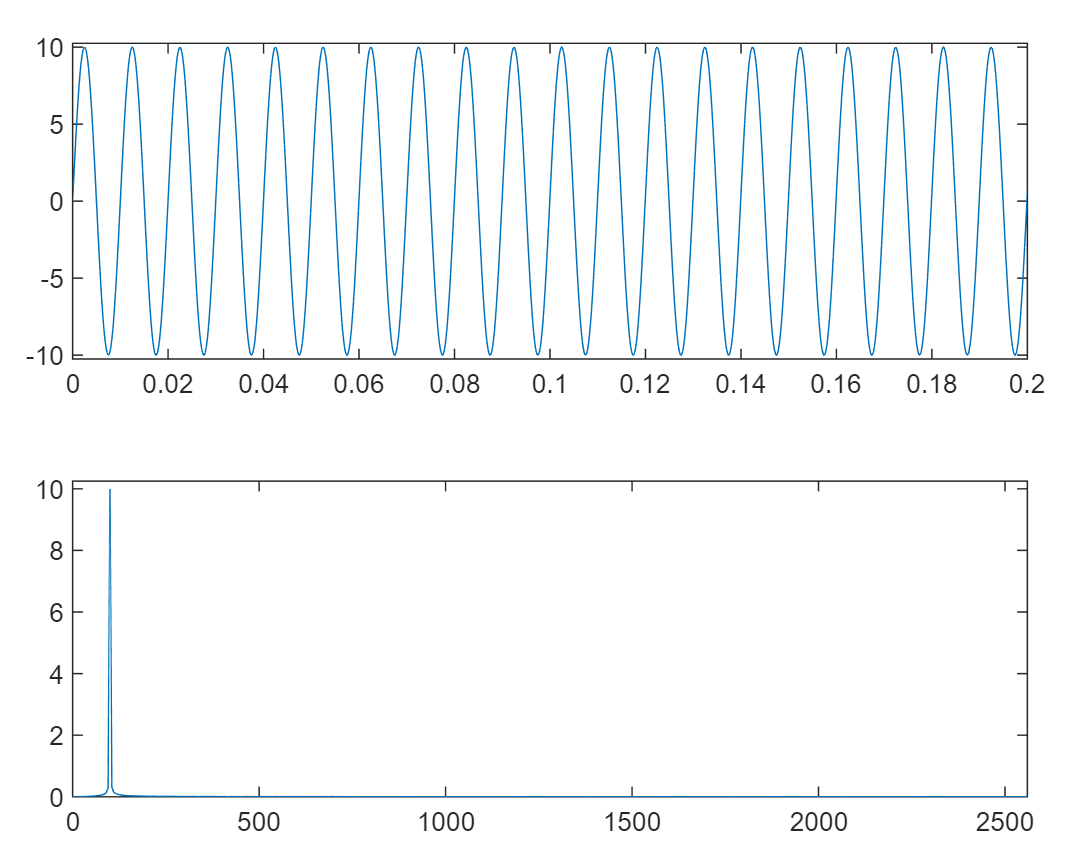
1. The sine wave signal with amplitude of 1 and frequency of 100.05Hz is sampled at a sampling rate of 5120Hz, and then 1024 point FFT is performed to display the signal waveform and spectrum; Observe the difference between signal waveform amplitude and spectrum amplitude, and analyze the reasons for the difference.

Fs = 5120;         % Adopted frequency
F = 100.05;            % signal frequency 
N = 1024;           % Sampling points
dt = 1/Fs;          % Sampling interval
T = dt*N;           % Total sampling time
t = linspace(0,T,N);% Sampling time
x = 10*sin(2*pi*F*t);
y = fft(x,N);
f = linspace(0,Fs/2,N/2);% x Coordinate conversion to frequency
figure
subplot(2,1,1)
plot(t,x)
axis([-inf,inf,-10.25,10.25]);
subplot(2,1,2)
plot(f,abs(y(1:N/2))/(N/2))
axis([-inf,inf,0,10.25]);

result:

reference resources:
Course:
Theory and practice of digital signal analysis -- Mr. He lingsong, Huazhong University of science and technology