[learning notes] polynomial logistic regression with numpy

Polynomial logistic regression is to add high-order terms as features on the basis of logistic regression to realize the extraction of high-dimensional features

Model construction

Polynomial logistic regression model is composed of three sub models:

(1) Add polynomial feature

(2) Standardization

(3) Logistic regression

Add polynomial feature

Multiply each feature to obtain a new feature. For example, the original feature is \ ([x_0,x_1] \)

Quadratic polynomials are characterized by \ ([1,x_0,x_1,x_0^2,x_0x_1,x_1^2] \)

Cubic polynomials are characterized by \ ([1,x_0,x_1,x_0^2,x_0x_1,x_1^2,x_0^3,x_0^2x_1,x_0x_1^2,x_1^3] \)

def poly_transform(X):
    XX=X.T
    ret=[np.repeat(1.0,XX.shape[1]),XX[0],XX[1]]
    for i in range(2,degree+1):
        for j in range(0,i+1):
            ret.append(XX[0]**(i-j)*XX[1]**j)
    return np.array(ret).T

Super parameter setting:

degree=3

Standardization

Scale the sample to a mean value of 0, a standard deviation of 1, and a transformation formula of \ (\ Large x=\frac{x-\mu}{\sigma} \)

Pit point:

(1) The standard deviation may be 0. When converting, the denominator will be 0, which needs to be converted to a non-zero number

(2) You only need to fit the training data once and transform it according to the mean and standard deviation during training, otherwise there will be deviation

def scaler_fit(X):
    global mean,scale
    mean=X.mean(axis=0)
    scale=X.std(axis=0)
    scale[scale<np.finfo(scale.dtype).eps]=1.0
def scaler_transform(X):
    return (X-mean)/scale

logistic regression

The core part of the model, the training process consists of three parts: forward propagation, loss calculation and back propagation:

Forward propagation

Calculate output probability from input data \ (p(x) \)

\[p(x)=\sigma(w^Tx) \]

def sigmoid(x):
    return 1/(1+exp(-x))
def forward(x):
    return sigmoid(w@x.T)

In a sense \ (p(x) \) represents the probability that \ (x \) is judged as class 1
It is reasonable to add an offset term \ (b \), which may be better for some data

Calculate loss

Suppose that the probability of training data \ (x \) \ (p=p(x) \) has been obtained in the previous step

For a single training data \ ([p,y] \), the loss function is:

\[J=-[y\log p+(1-y)\log(1-p)] \]

Using MBGD, multiple training data are obtained at one time. For a group of batch with m training data, the following are:

\[J=-\frac{1}{m}\sum_{i=0}^{m-1}[y_i\log p_i+(1-y_i)\log(1-p_i)] \]

In order to prevent the weight of \ (w \) from expanding excessively (because the greater the absolute value of each weight of \ (w \), the closer the value of \ (p \) is to 0 or 1), L1 regular term is added. Therefore, the final loss function is:

\[J=-\frac{1}{m}\sum_{i=0}^{m-1}[y_i\log p_i+(1-y_i)\log(1-p_i)]+k||w||_1 \]

def compute_loss(p,y):
    return np.mean(-(y*log(p)+(1-y)*log(1-p)),axis=0)+k*np.linalg.norm(w,ord=1)

Back propagation + update parameters

Calculate the partial derivative of each weight of loss function \ (J \) to \ (w \)

For convenience of thinking, consider only the case of single data \ ([p,y] \):

\[\frac{\part J}{\part p}=-(\frac{y}{p}-\frac{1-y}{1-p})\\ \frac{\part p}{\part(w^Tx)}=p(1-p)\\ \frac{\part(w^Tx)}{\part w_i}=x_i \]

So there

\[\frac{\part{J}}{\part{w_i}} =\frac{\part{J}}{\part{p}}\frac{\part{p}}{\part(w^Tx)}\frac{\part(w^Tx)}{\part w_i} =(p-y)x_i \]

For m training data:

\[\frac{\part{J}}{\part{w_i}}=\frac{1}{m}\sum_{j=0}^{m-1}(p_j-y_j)x_{ji} \]

After adding regular items:

\[\frac{\part{J}}{\part{w_i}}=\frac{1}{m}\sum_{j=0}^{m-1}(p_j-y_j)x_{ji}+k\text{sign}(w_i) \]

The form written as a vector is:

\[\frac{\nabla J}{\nabla w}=\frac{1}{m}\sum_{j=0}^{m-1}(p_j-y_j)x_{j}+k\text{sign}(w) \]

Update parameters while back propagating, i.e.:

\[w=w-\alpha\frac{\nabla J}{\nabla w} \]

\(\ alpha \) represents the learning rate

def backward(p,x,y):
    global w
    w-=learning_rate*np.mean((p-y).reshape(-1,1)*x,axis=0)+k*sign(w)

train

MBGD is used for training, and the learning rate is set as learning_rate, the weight of the regular item is k, and the training data scale of a batch is batch_size, the iteration round is epoch_num:

def logistic_fit(X,Y):
    global w
    XX=X.copy()
    YY=Y.copy()
    w=random.randn(XX[0].shape[0])*0.01
    I=list(range(len(XX)))
    LOSS=[]
    for epoch in range(epoch_num):
        random.shuffle(I)
        XX=XX[I]
        YY=YY[I]
        for i in range(0,len(XX),batch_size):
            x=XX[i:i+batch_size]
            y=YY[i:i+batch_size]
            p=forward(x)
            loss=compute_loss(p,y)
            LOSS.append(loss)
            backward(p,x,y)
    return LOSS

Super parameter setting:

learning_rate=0.9
k=0.005
batch_size=32
epoch_num=50

2, Generate training data

Generate training data sets \ (X \) and \ (Y \), where \ (X=\{x \} \), \ (Y=\{y \} \), \ (x=[x_0,F(x_0)] \), \ (x_0 ∈ [l,r] \), the label is \ (Y \), and the data set size is n

def generate_data(F,l,r,n,y):
    x=np.linspace(l,r,n)
    X=np.column_stack((x,F(x)))
    Y=np.repeat(y,n)
    return X,Y

Three, model training and prediction

train

Enter the training sample \ ((X,Y) \), update the parameters of scaler and logistic progression, and draw the loss curve with no return value

def train(X,Y):
    XX=poly_transform(X)
    scaler_fit(XX)
    XX=scaler_transform(XX)
    LOSS=logistic_fit(XX,Y)
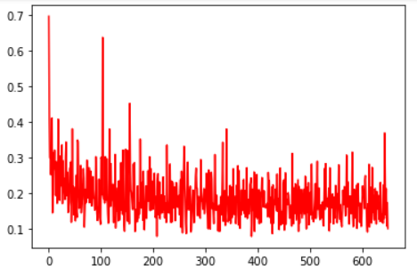
    plt.plot(list(range(len(LOSS))),LOSS,color='r')
    plt.show()

forecast

Enter the prediction sample \ (X \) and return the prediction result \ (\ hat Y \)

def predict(X):
    XX=scaler_transform(poly_transform(X))
    return logistic_predict(XX)

Draw discrimination interface

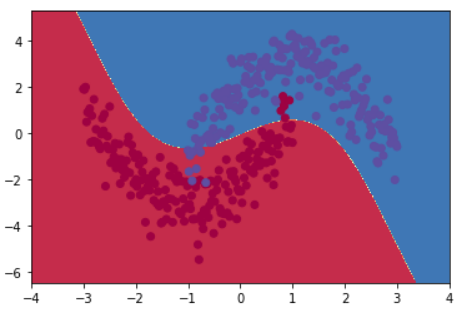
Input prediction sample \ ((X,Y) \), scatter diagram, and discrimination interface

def plot_decision_boundary(X,Y):
    global predY1
    x0_min,x0_max=X[:,0].min()-1,X[:,0].max()+1
    x1_min,x1_max=X[:,1].min()-1,X[:,1].max()+1
    m=500
    x0,x1=np.meshgrid(
        np.linspace(x0_min,x0_max,m),
        np.linspace(x1_min,x1_max,m)
    )
    XX=np.c_[x0.ravel(),x1.ravel()]
    Y_pred=predict(XX)
    Z=Y_pred.reshape(x0.shape)
    plt.contourf(x0,x1,Z,cmap=plt.cm.Spectral)
    plt.scatter(X[:,0],X[:,1],c=Y,cmap=plt.cm.Spectral)
    plt.show()

4, Main program

random.seed(114514)
data_size=200
X1,Y1=generate_data(lambda x:x**2+2*x-2+random.randn(data_size)*0.8,-3,1,data_size,0)
X2,Y2=generate_data(lambda x:-x**2+2*x+2+random.randn(data_size)*0.8,-1,3,data_size,1)
X=np.vstack((X1,X2))
Y=np.hstack((Y1,Y2))
train(X,Y)
plot_decision_boundary(X,Y)

loss curve:

Discrimination interface:

5, Complete code

Import dependent packages

import numpy as np
from numpy import exp,log,sign,random
from matplotlib import pyplot as plt

model building

# LogisticRegression
learning_rate=0.9
k=0.005
batch_size=32
epoch_num=50
def sigmoid(x):
    return 1/(1+exp(-x))
def forward(x):
    return sigmoid(w@x.T)
def compute_loss(p,y):
    return np.mean(-(y*log(p)+(1-y)*log(1-p)),axis=0)+k*np.linalg.norm(w,ord=1)
def backward(p,x,y):
    global w
    w-=learning_rate*np.mean((p-y).reshape(-1,1)*x,axis=0)+k*sign(w)
def logistic_fit(X,Y):
    global w
    XX=X.copy()
    YY=Y.copy()
    w=random.randn(XX[0].shape[0])*0.01
    I=list(range(len(XX)))
    LOSS=[]
    for epoch in range(epoch_num):
        random.shuffle(I)
        XX=XX[I]
        YY=YY[I]
        for i in range(0,len(XX),batch_size):
            x=XX[i:i+batch_size]
            y=YY[i:i+batch_size]
            p=forward(x)
            loss=compute_loss(p,y)
            LOSS.append(loss)
            backward(p,x,y)
    return LOSS
def logistic_predict(X):
    return np.where(forward(X)>0.5,1,0)
    
# StandardScaler
def scaler_fit(X):
    global mean,scale
    mean=X.mean(axis=0)
    scale=X.std(axis=0)
    scale[scale<np.finfo(scale.dtype).eps]=1.0
def scaler_transform(X):
    return (X-mean)/scale

# PolynomialFeatures
degree=3
def poly_transform(X):
    XX=X.T
    ret=[np.repeat(1.0,XX.shape[1]),XX[0],XX[1]]
    for i in range(2,degree+1):
        for j in range(0,i+1):
            ret.append(XX[0]**(i-j)*XX[1]**j)
    return np.array(ret).T

Model training and prediction

def train(X,Y):
    XX=poly_transform(X)
    scaler_fit(XX)
    XX=scaler_transform(XX)
    LOSS=logistic_fit(XX,Y)
    plt.plot(list(range(len(LOSS))),LOSS,color='r')
    plt.show()
def predict(X):
    XX=scaler_transform(poly_transform(X))
    return logistic_predict(XX)
def plot_decision_boundary(X,Y):
    global predY1
    x0_min,x0_max=X[:,0].min()-1,X[:,0].max()+1
    x1_min,x1_max=X[:,1].min()-1,X[:,1].max()+1
    m=500
    x0,x1=np.meshgrid(
        np.linspace(x0_min,x0_max,m),
        np.linspace(x1_min,x1_max,m)
    )
    XX=np.c_[x0.ravel(),x1.ravel()]
    Y_pred=predict(XX)
    Z=Y_pred.reshape(x0.shape)
    plt.contourf(x0,x1,Z,cmap=plt.cm.Spectral)
    plt.scatter(X[:,0],X[:,1],c=Y,cmap=plt.cm.Spectral)
    plt.show()

Generate training data

def generate_data(F,l,r,n,y):
    x=np.linspace(l,r,n)
    X=np.column_stack((x,F(x)))
    Y=np.repeat(y,n)
    return X,Y

main program

random.seed(114514)
data_size=200
X1,Y1=generate_data(lambda x:x**2+2*x-2+random.randn(data_size)*0.8,-3,1,data_size,0)
X2,Y2=generate_data(lambda x:-x**2+2*x+2+random.randn(data_size)*0.8,-1,3,data_size,1)
X=np.vstack((X1,X2))
Y=np.hstack((Y1,Y2))
train(X,Y)
plot_decision_boundary(X,Y)

reference material

[1] Machine learning: logistic regression (using polynomial features)
[2] Deep learning PyTorch minimalist tutorial

Keywords: Machine Learning

Added by kanikilu on Thu, 20 Jan 2022 02:15:55 +0200

Programming VIP

[learning notes] polynomial logistic regression with numpy

Model construction

Add polynomial feature

Standardization

logistic regression

Forward propagation

Calculate loss

Back propagation + update parameters

train

2, Generate training data

Three, model training and prediction

train

forecast

Draw discrimination interface

4, Main program

5, Complete code

reference material

Popular Keywords