Realization of convolutional neural network by TensorFlow

A course introduction

1.1 knowledge points

1. Introduction of convolutional neural network;
2. TensorFlow practices CNN network;

II. Course content

2.1 basic introduction of convolutional neural network

Convolution neural network is a neural network model constructed by convolution structure. Its characteristics are local perception, weight sharing, pooling, parameter reduction and multi-level structure.
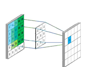
Its basic structure includes input layer, convolution layer, down sampling and fully connected output layer. Each layer is convoluted by the convolution check image. The calculated matrix is called the feature map, and the region mapped by the feature map in the original image is called the receptive field. Generally speaking, the receptive field size of the first convolution layer is equal to the convolution kernel size, while the receptive field size of the subsequent convolution layer is related to the size and step size of each convolution kernel before. The basic concepts of convolution kernel and step size are introduced below.

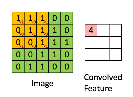
2.1.1 convolution kernel and step size

The convolution kernel includes the size of convolution kernel, the number of input channels and the number of output channels. For example, (5,5,32,64) means that 64 32 channel 5 * 5 convolution kernels are convoluted with the input to obtain 64 convolution results. Among them, the calculation of convolution is operated by multiplying and summing elements one by one. The length of each convolution movement is its convolution step.

Padding is also used in the concept of convolution kernel. That is, in order to solve the problem of smaller and smaller image and loss of boundary information in convolution operation. There are two types of padding:
(1) valid padding: only the original image is used without any processing, and the convolution kernel is not allowed to exceed the boundary of the original image;
(2) same padding: filling, allowing the convolution kernel to exceed the boundary of the original image, and making the size of the convolution result consistent with the original.

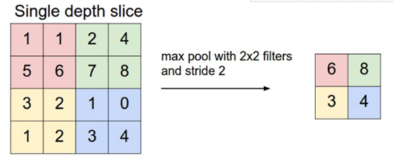
2.1.2 pooling

The role of pooling layer is to reduce the dimensions of each feature in order to reduce the amount of calculation. Generally speaking, the pool layer is often located behind each convolution layer to reduce the effect of calculation and prevent over fitting. The calculation method of the pool layer is similar to that of the convolution layer, which is the multiplication and addition of various elements. The difference is that the convolution kernel has training parameters, while the pool layer has no training parameters, just to reduce the calculation. The pool layer is divided into the following two categories:
(1) max pooling: select the largest element from the window correction diagram;
(2) average pooling: calculate the average from the window characteristic graph

2.1.3 CNN features

Local receptive field: convolutional neural network extracts local features by using convolution kernel, and then synthesizes the regional features felt by different neurons at a deep level, so as to obtain global information and reduce the number of connections.
Weight sharing: sharing parameters among different neurons can reduce the amount of calculation of the model, and weight sharing is to use the same convolution kernel for convolution operation on the image, so that all neurons in the convolution layer can detect the same features at different positions of the image, and its main function is to detect the same type of features at different positions, That is, the image can be translated in a small range, that is, translation invariance.

III. experimental test

3.1 predefined

First, import the Library:

import tensorflow as tf
from tensorflow.examples.tutorials.mnist import input_data

(1) Then read the handwritten font data set and convert it into onehot coding, that is, different image features are represented by different coding methods.

mnist = input_data.read_data_sets('MNIST_data_bak/', one_hot=True)

(2) Initialize the calculation session context. In TensorFlow, the calculation of numbers depends on the structure of the session:

sess = tf.InteractiveSession()

(3) Define the W variable in the model, comply with the initialization of positive distribution, and set the standard deviation to 0.1:

def weight_variable(shape):
    initial = tf.truncated_normal(shape, stddev=0.1)
    return tf.Variable(initial)

(4) Define b variables and initialize them as constants:

def bias_variable(shape):
    initial = tf.constant(0.1, shape=shape)
    return tf.Variable(initial)

(5) Define the convolution function, where x is the input image data, w is the convolution parameter, where stripe is the defined step size, and padding uses the same method:

def conv2d(x, W):
    return tf.nn.conv2d(x, W, strides=[1, 1, 1, 1], padding='SAME')

(6) Define the pooling layer function, where x is the input image data, w is the convolution parameter, where stripe is the defined step size (for the purpose of compressing data, the step size is 2), and padding uses the same method:

def max_pool_2x2(x):
    return tf.nn.max_pool(x, ksize=[1, 2, 2, 1], strides=[1, 2, 2, 1], padding='SAME')

3.2 model structure construction

(1) The input and output in TensorFlow need to be established by using placeholders. Because the size of the input image is 2828, it is necessary to convert the one-dimensional input vector into a two-dimensional picture structure, that is, from the form of 1784 to the original 28 * 28 structure.

x = tf.placeholder(tf.float32, [None, 784])
y_ = tf.placeholder(tf.float32, [None, 10])
x_image = tf.reshape(x, [-1, 28, 28, 1])

(2) Define the first convolution layer, where [3,3,1,32] represents that the convolution kernel size is 33, 1 color channel and 32 different convolution kernels, then use the conv2d function for convolution operation, add the bias term, then use the ReLU activation function for nonlinear processing, and finally use the maximum pooling function max_pool_22 pool the output results of convolution.

W_conv1 = weight_variable([3, 3, 1, 32])
b_conv1 = bias_variable([32])
h_conv1 = tf.nn.relu(conv2d(x_image, W_conv1) + b_conv1)
h_pool1 = max_pool_2x2(h_conv1)

(3) Define the second convolution layer, where [5,5,32,64] represents that the convolution kernel size is 55, 32 input channels and 64 convolution kernels with different outputs. Then use the conv2d function for convolution operation, add the bias term, and then use the ReLU activation function for nonlinear processing. Finally, use the maximum pool function max_pool_22 pool the output results of convolution.

W_conv2 = weight_variable([5, 5, 32, 64])
b_conv2 = bias_variable([64])
h_conv2 = tf.nn.relu(conv2d(h_pool1, W_conv2) + b_conv2)
h_pool2 = max_pool_2x2(h_conv2)

(4) Because we have experienced two times of maximum pooling with a step size of 22, the side length is only 1 / 4, and the picture size has changed from 2828 to 77. After two pooling, each pooling becomes 1 / 2. The number of convolution cores of the second convolution layer is 64, and the output tensor size is 77 * 64. We use TF The reshape function deforms the output tensor of the second convolution layer and converts it into a one-dimensional vector. Then connect a full connection layer with 1024 hidden nodes, and use ReLU activation function to combine features.

W_fc1 = weight_variable([7 * 7 * 64, 1024])
b_fc1 = bias_variable([1024])
h_pool2_flat = tf.reshape(h_pool2, [-1, 7 * 7 * 64])
h_fc1 = tf.nn.relu(tf.matmul(h_pool2_flat, W_fc1) + b_fc1)

(5) Use the softmax activation function for classification, and add and classify the full connection layer.

W_fc2 = weight_variable([1024, 10])
b_fc2 = bias_variable([10])
y_conv = tf.nn.softmax(tf.matmul(h_fc1, W_fc2) + b_fc2)

3.3 optimizer and loss function

Here, we use Adam loss function with a learning rate of 0.01 and cross entropy loss for classification.

cross_entropy = tf.reduce_mean(-tf.reduce_sum(y_ * tf.log(y_conv),
                                              reduction_indices=[1]))
train_step = tf.train.AdamOptimizer(1e-4).minimize(cross_entropy)

3.4 model iteration training and evaluation

(1) Set the accuracy of model calculation.

correct_prediction = tf.equal(tf.argmax(y_conv, 1), tf.argmax(y_, 1))
accuracy = tf.reduce_mean(tf.cast(correct_prediction, tf.float32))

(2) Model iterative training

accuracys=[]
tf.global_variables_initializer().run()
for i in range(1000):
    batch = mnist.train.next_batch(50)
    if i % 10 == 0:
        train_accuracy = accuracy.eval(feed_dict={x: batch[0], y_: batch[1]})
        print("step : %d, |training accuracy : %g" % (i, train_accuracy))
        accuracys.append(train_accuracy)
    train_step.run(feed_dict={x: batch[0], y_: batch[1]})

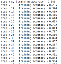
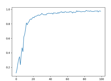
3.5 visual drawing

Draw the evaluation chart according to the accuracy.

import matplotlib.pyplot as plt
plt.plot(accuracys)
plt.show()

IV. thinking and homework

(1) Try to tune the model (from the aspects of learning rate, batch size and model structure)
(2) Try to use TensorFlow to realize training to generate pictures, that is, input text 1 to generate picture 1