introduction

Linear regression may be the earliest machine learning algorithm we came into contact with. In the high school mathematics textbook, we officially knew this friend for the first time. We obtained the linear regression equation of the data through the least square method, and then obtained the parameters of the model. But in fact, in junior high school, we learned the skill of solving a function through the coordinates of two known points, which is also a special case of linear regression model. Today, let's introduce another method for solving linear regression model - gradient descent method.

Introduction to linear regression

• Linear regression definition

Linear regression is an analytical method that uses regression equation (function) to model the relationship between one or more independent variables (eigenvalues) and dependent variables (target values).

• for instance

Lao Huang worked diligently for several n years and finally saved some money to buy a house ~ the statistics of a real estate are as follows:

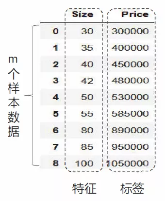
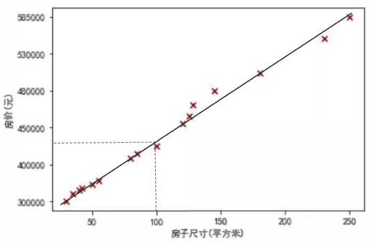
Drawing these data points on the coordinate axis, we can see that the house area and house price are roughly linear distribution, that is, they are roughly distributed in a straight line. If we can find the equation of this straight line, we can predict the price of a house according to its area.

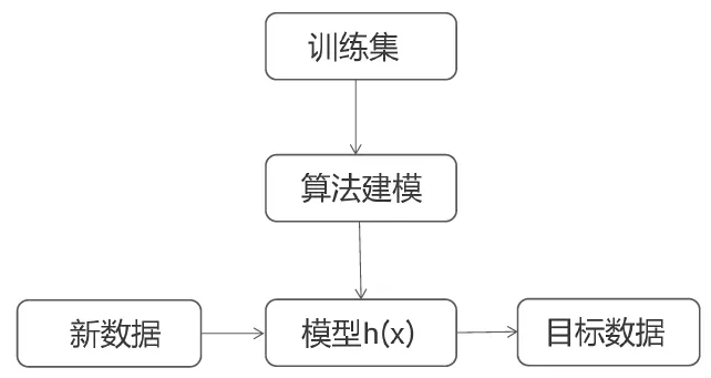
The simplified process of linear regression is as follows

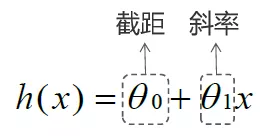
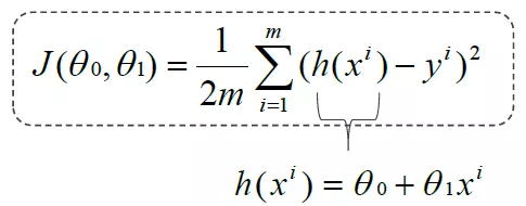
Where h(x) is:

Objective: to find the best fitting line to minimize the error, that is, the cost function. The cost function is:

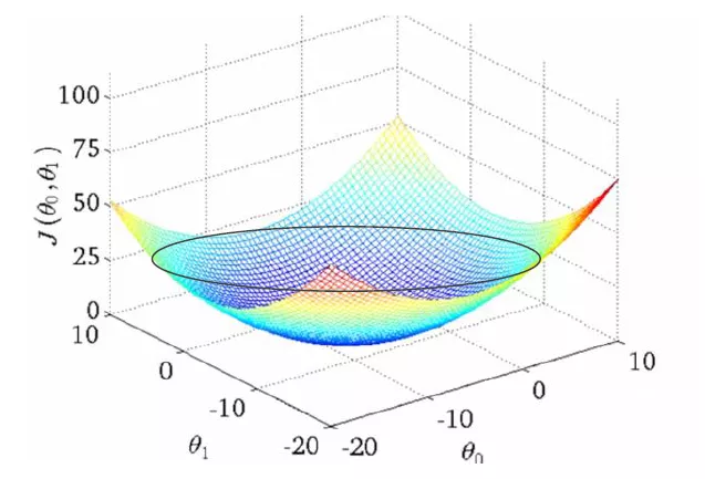
Cost function and θ 0 θ The relationship of 1 is shown in the figure:

• Introduction to gradient descent method

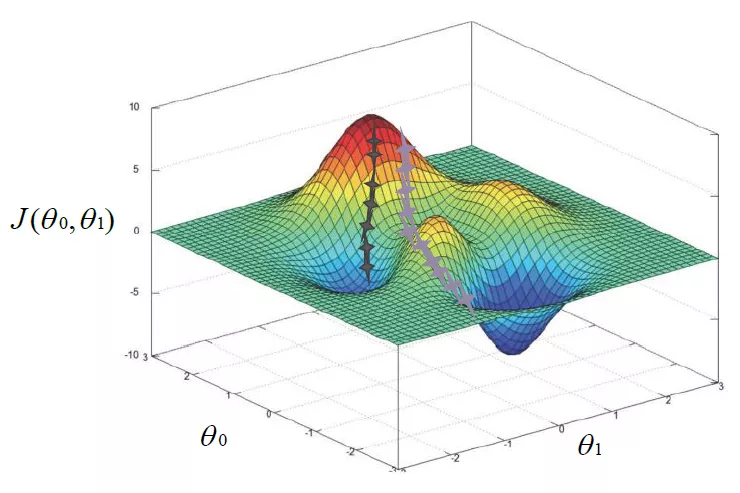
Gradient descent method is an algorithm that can minimize the cost function, that is, to find the appropriate cost function θ 0 θ 1 makes the cost function J( θ 0 θ 1) The minimum implementation steps are:
1. Initialization θ 0 θ 1；
2. Keep changing θ 0 θ 1 makes J( θ 0 θ 1) Decrease;
3. Until J( θ 0 θ 1) Minimum or local minimum of.

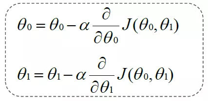
Repeat the following:

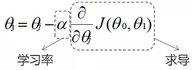
Update at the same time:

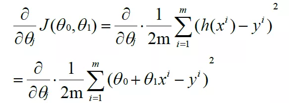
Substitute h(x) into the equation to obtain:

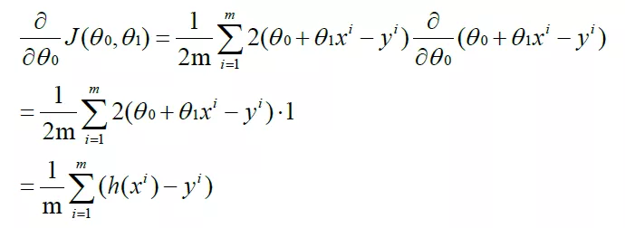
yes θ 0 partial derivative:

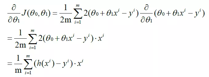
yes θ 1. Partial derivation:

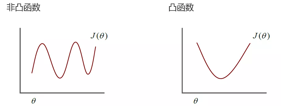
For convex functions, the gradient descent method can generally get the unique optimal solution, and for non convex functions, it may fall into the local optimal solution.

Next, we use numpy to manually implement gradient descent linear regression, and then call sklearn interface to realize linear regression.

Manual implementation of gradient descent linear regression

1. Import libraries that may need to be used, import csv data files, define x variables and y variables, and plot the distribution of X and y data.

import numpy as np
import matplotlib.pyplot as plt
plt.rcParams['font.sans-serif'] = ['SimHei'] # Step 1 (replace sans serif font)
plt.rcParams['axes.unicode_minus'] = False   # Step 2 (solve the problem of negative sign display of coordinate axis negative numbers)

data = np.loadtxt('data.csv',delimiter=',')
x_data = data[:,0]
y_data = data[:,1
plt.scatter(x_data,y_data,marker='x',color='red')
plt.show()

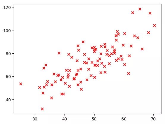
The output results are as follows. It can be seen that x and y show roughly linear distribution.

2. Define the learning rate, initial intercept and slope, number of iterations, and define the calculation method of cost function

learning_rate = 0.0001
b = 0
k = 0
n_iterables = 50

def compute_mse(x_data,y_data,k,b):
    mse = np.sum((y_data-(k*x_data+b))**2)/len(x_data)/2
    return mse

3. To define the gradient descent function, you need to import x, y, initial intercept, initial slope, learning rate and iteration times as parameters, and the final output results are target intercept, target slope and cost function value list.

def gradient_descent(x_data,y_data,k,b,learning_rate,n_iterables):
    m = len(x_data)
    start_loss = compute_mse(x_data,y_data,k,b)
    loss_value = [start_loss]
    for i in range(n_iterables):
        b_grad = np.sum((k*x_data+b)-y_data)/m
        k_grad = np.sum(((k*x_data+b)-y_data)*x_data)/m
        b = b - (learning_rate*b_grad)
        k = k - (learning_rate*k_grad)
        loss_value.append(compute_mse(x_data,y_data,k,b))
        print(b,k)
    return b,k,np.array(loss_value)

4. Call the function to get the result and draw.

b1,k1,loss_list = gradient_descent(x_data,y_data,k,b,learning_rate,n_iterables)
y_predict = k1*x_data+b1
print(b1,k1)

plt.scatter(x_data,y_data,marker='x',color='red')
plt.plot(x_data,y_predict)
plt.show()

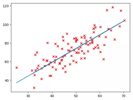
Output result b1=0.03056, k1=1.47889
As shown in the picture, it looks ok.

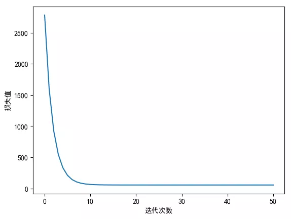
5. Draw the curve of the cost function with the number of iterations, as shown in the figure. It can be seen that after 10 iterations, the change of the cost function is relatively small.

plt.plot(range(n_iterables+1),loss_list)
plt.xlabel('Number of iterations')
plt.ylabel('magnitude of the loss')
plt.show()

Call API interface to realize linear regression

1. Similarly, import libraries that may need to be used, import csv data files, define x variables and y variables, and draw and display the distribution of X and y data.

import numpy as np
from sklearn.linear_model import LinearRegression
import matplotlib.pyplot as plt

data = np.loadtxt('data.csv',delimiter=',')
x_data = data[:,0,np.newaxis]
y_data = data[:,1]
plt.scatter(x_data,y_data,marker='x',color='red')
plt.show()

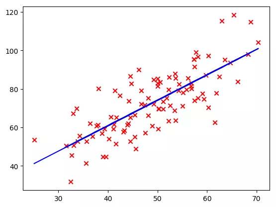
2. Define the model, fit it, predict it, get the results and draw it. It can be seen that the steps of calling API interface are very simple.

model = LinearRegression()
model.fit(x_data,y_data)
y_predict = model.predict(x_data)
plt.scatter(x_data,y_data,marker='x',color='red')
plt.plot(x_data,model.predict(x_data),'b')
plt.show()

3. Printout intercept and slope

b = model.intercept_
k = model.coef_[0]
print(b,k)

Output: b=7.99102, k=1.322431. There is still some difference from the above results, because the above only iterates 50 times, and the exact solution is obtained by calling the interface.

Little buddy, have you learned? Scan the bottom two dimensional code to pay attention to the official account, and get the data and source code back to the "linear regression 1" in the background.