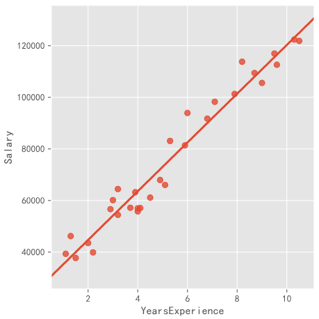
Univariate linear regression model:

E: Model Error Term, Equilibrium Equal Side Value

import seaborn as sns
income = pd.read_csv(r'Salary_Date.csv')
sns.lmplot(x='YearExperience',y='Salary',
			data=income,ci=None)
plt.show()

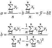
Linear fitting solution:
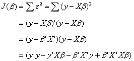
Minimum Error Term and Minimum Conversion to Minimum Square Error Term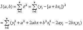

At the minimum, the partial derivative is 0.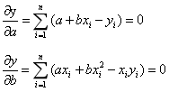


Using Basic Grammar to Solve

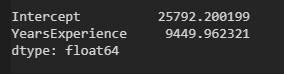
n = income.shape[0]
sum_x = income.YearsExperience.sum()
sum_y = income.Salary.sum()
sum_x2 = income.YearsExperience.pow(2).sum()
xy = income.YearsExperience * income.Salary
sum_xy = xy.sum()
b = (sum_xy - sum_x * sum_y / n) / (sum_x2 - sum_x ** 2 / n)
a = sum_y.mean() - b * sum_x.mean()

(2) Using ols function in statsmodels
ols(formula,data,subset=None,drop_cols)
formula: 'y~x'
Subset: bool type, subset modeling

import statsmodels.api as sm
fit = sm.formula.ols('income.Salary ~ income.YearsExperience',data=income).fit()
fit.params

multiple linear regression

The data set of multivariate linear regression consists of n observations and p+1 variables (p independent variables and 1 dependent variable).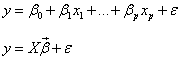

One-dimensional Vector of Beta:p1, Partial Regression Coefficient
One-Dimensional Vector of E:n1, Error Term

Constant, transposed to itself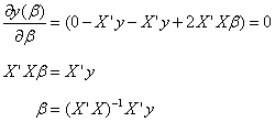

Prodict_Profit.xlsx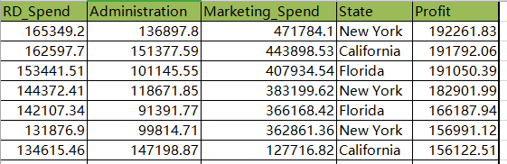

State is a character discrete variable

from sklearn import model_selection
import statsmodels.api as sm
profit = pd.read_excel(r'Prodict_Profit.xlsx')
train,test = model_selection.train_test_split(profit,test_size=0.2,random_state=1234)
model = sm.formula.ols('Profit ~ RD_Spend + Administration + Marketing_Spend + C(State)',data=train).fit()
print(model.params)
test_X = test.drop(labels='Profit',axis=1)
pred = model.predict(exog=test.X)
print({'prediction':pred,'real':test.Porfit})

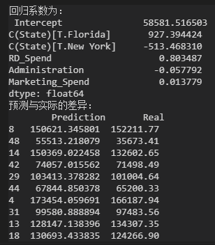
State is a discrete variable, dumb variable, nested in C(), expressed as category variable.
State: Cal, Flo, NY. Cal was used as the control group by default in the model.

NY as control group

dummies = pd.get_dummies(profit.State)
profit_new = pd.concat([profit,dummies],axis=1)
profit_new.drop(labels=['State','New York'],axis=1,inplace=True)
train,test = model_selection.train_test_split(profit_new,test_size=0.2,random_state=1234)
model2 = sm.formula.ols('Profit ~  RD_Spend + Administration + Marketing_Spend + Flo + Cal',data=train).fit()
print(model2.params)

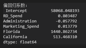
Dummy variables evolved from state retain only Flo and Al in the regression coefficients, while NY serves as the reference group.
Take RD_Spend and Fla as examples: with other variables unchanged, R&D cost increases by 1 yuan and profit increases by 0.8 yuan; with NY as the benchmark, sales in Flo increases by 1440 yuan.

Hypothesis Test of Regression Model

The saliency test of the model is whether the linear combination of dependent variables is effective, that is, whether there is an independent variable in the model can really affect the fluctuation of dependent variables and the overall effect.
The significance test of regression coefficient is to show whether a single independent variable is valid in the model.

The significance of model and regression coefficient were tested by F test and t test respectively.

1. F test

(1) Putting forward the original hypothesis and alternative hypothesis of the question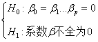

Overthrow H0 by data and accept H1
(2) Constructive statistics

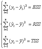
ESS: sum of squares of errors, varying with time
RSS: The sum of squares of regression deviations, varying with time
TSS: Total sum of squares of deviations, unchanged
TSS=ESS+RSS
The parameters of linear regression model are solved to minimize ESS and maximize RSS.

Constructing F-statistics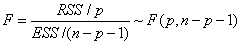

p: RSS degree of freedom
n-p-1:ESS degree of freedom

③

import numpy as np
ybar = train.Profit.mean()
p = model2.df_model
n = train.shape[0]
RSS = np.sum((model2.fittedvalues - ybar) **2)
ESS = np.sum(model2.resid **2)
F = (RSS / p) / (ESS / (n-p-1))
print(F)

#Verify that the manually calculated values are correct
model2.fvalue

(4) Comparing the value of F statistics with the value of theoretical F distribution

#Call to calculate the theoretical distribution value
from scipy.stats import f
F_throry = f.ppf(q=0.95,dfn=p,dfd=n-p-1)
print(F_theory)

The value of F statistic is much larger than the theoretical value of F distribution, so the original hypothesis is rejected and the multivariate linear regression model is considered to be significant, so the partial regression coefficient of the regression model is not all 0.

1. Significance test and t test of regression coefficient
   (1) Presenting hypotheses
   
   The original hypothesis is that the partial regression coefficient of the j variable is 0.

(2) Constructive statistics

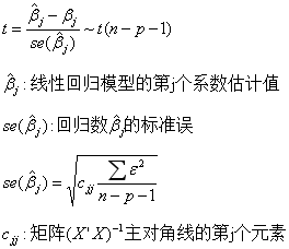
(3) Computational statistics

model2.summary()

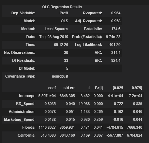
Part I:
The Decision Coefficient R-square of the Model: The Explanation Degree of Independent Variables to Dependent Variables
F-statistic of the model: testing the significance of the model
Model Information Criteria AIC, BIC: Comparing the Fitting Effect of the Model
Part II:
Estimates of regression coefficients Coef, t statistics, confidence intervals of regression coefficients
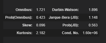
The third part:
Relevant information of model error term e, Durbin-Watson statistic to test the independence of error term, JB statistic to measure whether the error term obeys normal distribution, Skew of error term, Kurtosis of Kurtosis

(4) The second part contains t-statistics of each partial regression coefficient, which is derived from the quotient of estimated Coef and standard error Std err. Each t-statistics corresponds to the probability value P. It is a direct method to judge whether the statistics are significant or not. Generally, when the probability p is less than 0.05, it denies the original hypothesis and fails to indicate that the variables are not important factors.

After passing the test, the model was diagnosed.

Diagnosis of Regression Model

The hypothesis of the model requires normal distribution for residual items, and the essence requires that dependent variables obey normal distribution.
Normality test uses two methods:
Qualitative Graphic Method
Quantitative Nonparametric Method

(1) Histogram method

import scipy.stats as stats
plt.rcParams['font.sans-serif'] = ['SimHei']
plt.rcParams['axes.unicode-minus'] = False
plt.style.use('ggplot')
sns.distplot(a=profit_new.Profit,bins=10,fit=stats.norm,norm_hist=True,
				hist_kws=['color':'steelblue','edgecolor':'blue'],
				kde_kws=['color':'orange','linestyle':'-','label':True],
				fit_kws=['color':red,'linestyle':'--'])
plt.legend()
plt.show()

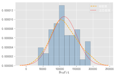
Draw the histogram of the variable Profit, the nuclear density curve, and the theoretical normal distribution. If the two curves are approximate or coincident, the normal distribution is obeyed.

PP chart, QQ chart

#Normal Test of Residual
import ststamodels.api as sm
pp_qq_plot = sm.ProbPlot(profit_new.Profit)
#PP diagram
pp_qq_plot.ppplot(line=45)
plt.title('PP chart')
pp_qq_plot.qqplot(line='q')
plt.title('QQ chart')
plt.show()

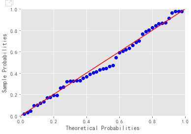
PP chart: Comparing the cumulative probability of normal distribution with the cumulative probability of actual distribution
QQ Diagram: Quantiles Contrasting Normal Distribution and Century Distribution
Criteria for judging whether variables obey normal distribution: scatters are fairly uniform on a straight line.

③Shapiro K-S
Assuming that the variables obey normal distribution, if the data is less than 5000, shapiro test is used.

import scipy.stats as stats
stats.shapiro(profit_new.Profit)

Returning to tuple, the first element is the statistical value of shapiro test and the second element is the corresponding probability P. Since the p value is greater than the confidence level of 0.05, it accepts that the profit distribution obeys the normal distribution.

#Generating Normal Distribution and Uniform Distribution
rnorm = np.random.normal(loc=5,scale=2,size=1000)
runif = np.random.unifrom(low=1,high=100,size=1000)
#Normality test
KS_test1 = stats.kstest(rvs=rnorm,args=(rnorm.mean(),rnorm.std()),cdf='norm')
KS_test2 = stats.kstest(rvs=runif,args=(runif.mean(),runif.std()),cdf='norm')

The test p value of the random number of normal random distribution is greater than 0.05 confidence level. Accept the original hypothesis.
p value of uniform distribution is less than 0.05, rejecting the original hypothesis
When using kstest function to test the normality of variables, args parameters must be specified, and the mean and standard deviation of the tested variables must be transmitted.
The results of variable test do not satisfy the normal distribution and use mathematical transformation.