Loan risk prediction

Loan default risk prediction

The project comes from the Kaggle competition. It is required to predict whether the customer's loan will default according to the customer's credit card information, installment information, credit bureau information and so on.

Load module and build environment

import numpy as np
import pandas as pd
import matplotlib.pyplot as plt
plt.rcParams['font.sans-serif'] = ['SimHei']

import seaborn as sns
import warnings
# Ignore warning
warnings.filterwarnings("ignore")
# IPython magic function, embedded drawing, PLT can be omitted Show() to display the image directly
%matplotlib inline

CSV data reading

train=pd.read_csv(r"C:\Users\TP\Desktop\myself\Loan risk\Credit risk data set\application_train.csv")
test=pd.read_csv(r"C:\Users\TP\Desktop\myself\Loan risk\Credit risk data set\application_test.csv")
train.sample(10)

	SK_ID_CURR	TARGET	NAME_CONTRACT_TYPE	CODE_GENDER	FLAG_OWN_CAR	FLAG_OWN_REALTY	CNT_CHILDREN	AMT_INCOME_TOTAL	AMT_CREDIT	AMT_ANNUITY	...	FLAG_DOCUMENT_18	AMT_REQ_CREDIT_BUREAU_HOUR	AMT_REQ_CREDIT_BUREAU_DAY	AMT_REQ_CREDIT_BUREAU_WEEK	AMT_REQ_CREDIT_BUREAU_MON	AMT_REQ_CREDIT_BUREAU_QRT	AMT_REQ_CREDIT_BUREAU_YEAR
74327	186199	0	Cash loans	M	N	Y	0	157500.0	640080.0	24259.5	...	0	0.0	1.0	1.0	0.0	0.0	1.0
105101	221958	0	Cash loans	F	N	Y	0	247500.0	1288350.0	37795.5	...	0	0.0	0.0	0.0	0.0	0.0	3.0
89301	203680	0	Revolving loans	M	Y	Y	0	225000.0	225000.0	11250.0	...	0	0.0	0.0	0.0	0.0	0.0	0.0
185992	315612	1	Cash loans	F	Y	Y	1	225000.0	562500.0	30645.0	...	0	0.0	0.0	0.0	0.0	0.0	2.0
254717	394747	0	Cash loans	F	N	Y	0	202500.0	405000.0	24601.5	...	0	0.0	0.0	0.0	0.0	1.0	2.0
57672	166832	0	Cash loans	M	N	N	2	157500.0	427450.5	23319.0	...	0	0.0	0.0	0.0	0.0	2.0	4.0
196040	327318	0	Cash loans	M	Y	N	0	112500.0	276277.5	14233.5	...	0	NaN	NaN	NaN	NaN	NaN	NaN
70982	182323	0	Cash loans	F	N	Y	1	117000.0	271066.5	13968.0	...	0	0.0	0.0	0.0	0.0	0.0	1.0
156304	281183	0	Revolving loans	F	N	N	1	90000.0	270000.0	13500.0	...	0	0.0	0.0	0.0	0.0	0.0	1.0
149247	273036	0	Cash loans	M	N	Y	2	144000.0	562500.0	26064.0	...	1	0.0	0.0	0.0	0.0	0.0	1.0

10 rows × 122 columns

Data cleaning

Missing value and abnormal value handling

Missing value

# Missing value detection, function definition
def mis_val(data):
    mis_val=data.isnull().sum().reset_index().rename(columns={"index":"feature",0:"mis_tol"})
    l=len(mis_val)
    mis_val["mis_per"]=(mis_val.mis_tol/len(data)*100).round(1)
    mis_nol=len(mis_val[mis_val.mis_tol==0])
    mis_num=len(mis_val[mis_val.mis_tol != 0])
    mis=mis_val[mis_val.mis_tol != 0].sort_values("mis_tol",ascending=False,ignore_index=True)
    print("Total yes"+str(l)+"column,\n"
         "among"+str(mis_nol)+"Column has no missing value,\n"
         "surplus"+str(mis_num)+"Column has missing values.")
    return mis

mis_val(train)

There are 122 columns in total,
There are no missing values in 55 columns,
The remaining 67 columns have missing values.

	feature	mis_tol	mis_per
0	COMMONAREA_MEDI	214865	69.9
1	COMMONAREA_AVG	214865	69.9
2	COMMONAREA_MODE	214865	69.9
3	NONLIVINGAPARTMENTS_MEDI	213514	69.4
4	NONLIVINGAPARTMENTS_MODE	213514	69.4
...	...	...	...
62	EXT_SOURCE_2	660	0.2
63	AMT_GOODS_PRICE	278	0.1
64	AMT_ANNUITY	12	0.0
65	CNT_FAM_MEMBERS	2	0.0
66	DAYS_LAST_PHONE_CHANGE	1	0.0

67 rows × 3 columns

Since the LGB model we use later is not sensitive to missing values, in order to simplify the process, the missing values will not be interpreted here. For some cases with the same missing rate of columns, further analysis is needed, and further processing will be carried out in the feature engineering part. If other models sensitive to missing values are used, the columns with missing values need to be processed one by one. The common processing methods of missing values include: delete and fill;

Outliers

Outliers: sometimes the dataset contains one or more values with abnormally large or small values. Such extreme values are called outliers
There are many ways to judge and deal with outliers, such as 3 Sigma method, percentile method, MAD method and so on
Here, we take the simplest method to describe statistics, that is, to view the mean, maximum, minimum and other information of the characteristics, and judge whether there are abnormal values in combination with the actual business

View the data distribution of user age

(train["DAYS_BIRTH"]/-365).describe()

count    307511.000000
mean         43.936973
std          11.956133
min          20.517808
25%          34.008219
50%          43.150685
75%          53.923288
max          69.120548
Name: DAYS_BIRTH, dtype: float64

It is found that the distribution of data is relatively normal. The maximum age is 69 years old and the minimum age is 20 years old. There are no very abnormal figures

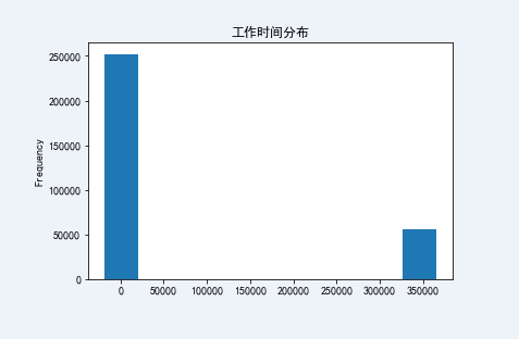
View the working time distribution of users and find

(train['DAYS_EMPLOYED']/-365).describe()

count    307511.000000
mean       -174.835742
std         387.056895
min       -1000.665753
25%           0.791781
50%           3.323288
75%           7.561644
max          49.073973
Name: DAYS_EMPLOYED, dtype: float64

The minimum value is - 1000 years, which is obviously an abnormal data. No one's working hours are negative, which is an abnormal value

# View working hours days_ Employee data distribution
train['DAYS_EMPLOYED'].plot.hist(title = 'Working time distribution')

<matplotlib.axes._subplots.AxesSubplot at 0x2b1a78e0>

Here, null values are used to replace outliers (whether 0 value, average value, median, etc. will change the data distribution, and LGB model allows the data to be null)

train['DAYS_EMPLOYED'].replace({365243: np.nan}, inplace = True)
(train['DAYS_EMPLOYED']/-365).plot.hist(title = 'Working time distribution')

<matplotlib.axes._subplots.AxesSubplot at 0x2be6ff70>

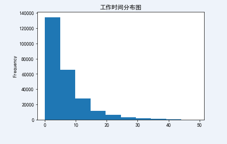
The outliers are erased. After replacement, let's take a look at the distribution of working hours. It's much normal

View the gender distribution of users and find

train.groupby("CODE_GENDER").size()

CODE_GENDER
F      202448
M      105059
XNA         4
dtype: int64

It is found that there is an abnormal value "XNA" in the user's gender. Since there are only four abnormal values, whether they are replaced by null values, F and m, they will not affect the result model and prediction results, so fill in M for the time being

train.CODE_GENDER.replace("XNA","M",inplace=True)
train.groupby("CODE_GENDER").size()

CODE_GENDER
F    202448
M    105063
dtype: int64

Check the service life distribution of the customer's car and find

train.OWN_CAR_AGE.describe()

count    104582.000000
mean         12.061091
std          11.944812
min           0.000000
25%           5.000000
50%           9.000000
75%          15.000000
max          91.000000
Name: OWN_CAR_AGE, dtype: float64

sns.set_style("darkgrid")
sns.boxplot(x=train.OWN_CAR_AGE,orient="v",width=0.3)

<matplotlib.axes._subplots.AxesSubplot at 0x290830d0>

If we judge the abnormal value according to the upper limit of the box diagram, the service life of the customer's car greater than 30 is the abnormal value. The actual business needs to be combined with the actual situation. The outlier limit is not necessarily 30. In this exercise, we tentatively set the upper limit of the box chart as the outlier limit;

# We fill the outliers with the upper boundary, which is 30
train.OWN_CAR_AGE[train.OWN_CAR_AGE>30]=30
# Note that if it is written as train [train. Own_car_age > 30] OWN_ CAR_ Age = 30 does not replace any data, and the reason is unknown

In actual business, abnormal value detection and processing should be carried out for each feature, and existing abnormal value processing functions / modules should be defined or adopted. Here, the process is simplified and will not be handled one by one;

Exploration of default user portrait

The goal of this part of analysis is to check the characteristic distribution of defaulting users and non defaulting users. The goal is to establish a basic understanding of the portrait of defaulting users and lay a foundation for subsequent feature engineering. For example, there are many fields in the data set, including gender, age, working hours, etc. are men more likely to default or women? Are older people more likely to default or younger people? Viewing these data can help us have a better understanding of the data. At the same time, if a field is not sensitive to the characteristic distribution of whether the user defaults, we can consider whether to delete this field.

Chart function definition

Define discrete chart functions

def discrete_bar(data,label,n=10):
    # Calculate label default rate
    group_label_0=data.groupby(label).TARGET.agg(["sum","count"])
    group_label_1=group_label_0.reset_index()
    group_label_1.columns=[label,"TARGET_SUM","TARGET_COUNT"]
    group_label_1["Default_Rate"]=(group_label_1["TARGET_SUM"]/group_label_1["TARGET_COUNT"]*100).round(2)
    group_label_1.sort_values(by="Default_Rate",ascending=False,inplace=True,ignore_index=True)
    print(group_label_1)
    # The chart shows that the histogram is used when the discrete value is small
    if len(group_label_1)<n:
        plt.figure(figsize=(14,8))
        sns.set_style("darkgrid")

        # label quantity distribution of each category
        plt.subplot(1,2,1)
        ax0=sns.barplot(x=label,y="TARGET_COUNT",data=group_label_1)
        ax0.set_xticklabels(group_label_1[label],rotation=45)
        x0=group_label_1[label]
        y0=group_label_1["TARGET_COUNT"]
        for  i ,j in zip(np.arange(len(x0)),y0):
            plt.text(i,j+np.mean(y0)/50,j,horizontalalignment="center")

        # Distribution chart of default rate of label
        plt.subplot(1,2,2)
        ax1=sns.barplot(x=label,y="Default_Rate",data=group_label_1)
        ax1.set_xticklabels(group_label_1[label],rotation=45)
        x1=group_label_1[label]
        y1=group_label_1["Default_Rate"]
        for  i ,j in zip(np.arange(len(x1)),y1):
            plt.text(i,j+0.2,j,horizontalalignment="center")

    # The chart shows that the bar chart is used when there are many discrete values
    else:
        plt.figure(figsize=(16,10))
        sns.set_style("whitegrid")

        # label quantity distribution of each category
        plt.subplot(1,2,1)
        ax0=sns.barplot(x="TARGET_COUNT",y=label,data=group_label_1,orient="h")
        ax0.set_yticklabels(group_label_1[label],rotation=75)
        x0=group_label_1[label]
        y0=group_label_1["TARGET_COUNT"]
        for  i ,j in zip(np.arange(len(x0)),y0):
            plt.text(j+np.mean(y0)/5,i,j,horizontalalignment="center")

        # Distribution chart of default rate of label
        plt.subplot(1,2,2)
        ax1=sns.barplot(x="Default_Rate",y=label,data=group_label_1,orient="h")
        ax1.set_yticklabels(group_label_1[label],rotation=75)
        x1=group_label_1[label]
        y1=group_label_1["Default_Rate"]
        for  i ,j in zip(np.arange(len(x1)),y1):
            plt.text(j+1,i,j,horizontalalignment="center")

Define continuous chart functions

def continuous_plot(data,label,cutn=8):
    plt.figure(figsize=(12,12))
    
    # Draw the nuclear density curve of default users and normal users
    plt.subplot(2,1,1)
    sns.set_style("darkgrid")
    sns.kdeplot(data[label][data["TARGET"]==0])
    sns.kdeplot(data[label][data["TARGET"]==1])
    
    # Segment the fields to calculate the default rate
    lb=data[[label,"TARGET"]]
    nln=label+"_CUT"
    lb[nln]=pd.cut(lb[label],cutn)
    lb_group=lb.groupby(nln)["TARGET"].agg(["sum","count"])
    lb_group["pro"]=(lb_group["sum"]/lb_group["count"]*100).round(2)
    lb_group.reset_index(inplace=True)
    print("Default rate of each segment\n\n",lb_group)
    plt.subplot(2,1,2)
    ax=sns.barplot(x=nln,y="pro",data=lb_group)
    ax.set_xticklabels(lb_group[nln],rotation=45)

Unified chart function

def chart_fuc(data,label,con_ornot="dispersed",n=10,cutn=8):
    if con_ornot=="dispersed":
        discrete_bar(data,label,n)
    elif con_ornot=="continuity" :
        continuous_plot(data,label,cutn)

Feature distribution image of each field

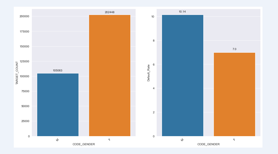
First, let's take a look at the default rate of male and female users. It is found that the default rate of male users is higher, with 10.14% for male users and 7% for women

chart_fuc(train,"CODE_GENDER")

  CODE_GENDER  TARGET_SUM  TARGET_COUNT  Default_Rate
0           M       10655        105063         10.14
1           F       14170        202448          7.00

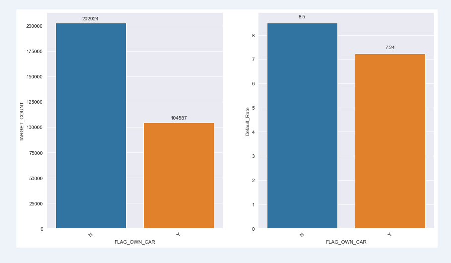
The default rate of users with cars is lower than that of users without cars. The default rate of users with cars is 7.24% and that of users without cars is 8.5%;

chart_fuc(train,"FLAG_OWN_CAR")

  FLAG_OWN_CAR  TARGET_SUM  TARGET_COUNT  Default_Rate
0            N       17249        202924          8.50
1            Y        7576        104587          7.24

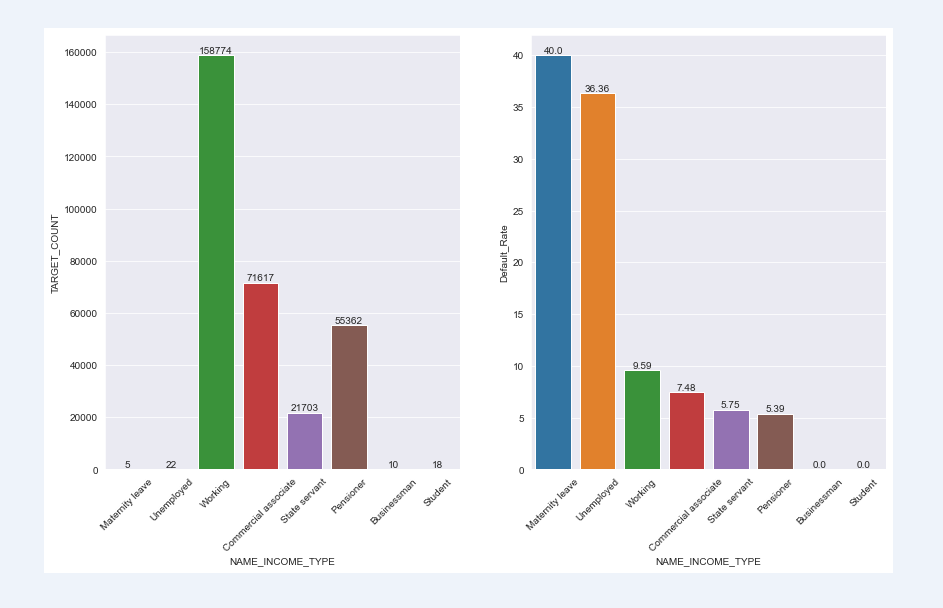
The default rate varies significantly with different types of user income; The default rate of employees taking maternity leave and unemployed is significantly higher than that of other income groups, among which the default rate of businessmen and students is 0;

chart_fuc(train,"NAME_INCOME_TYPE")

       NAME_INCOME_TYPE  TARGET_SUM  TARGET_COUNT  Default_Rate
0       Maternity leave           2             5         40.00
1            Unemployed           8            22         36.36
2               Working       15224        158774          9.59
3  Commercial associate        5360         71617          7.48
4         State servant        1249         21703          5.75
5             Pensioner        2982         55362          5.39
6           Businessman           0            10          0.00
7               Student           0            18          0.00

Users have different occupational types and different default rates, among which the default rate of low skilled workers is the highest, as high as 17.15%; The professional default rate of Accountants is the lowest, only 4.83%

chart_fuc(train,"OCCUPATION_TYPE")

          OCCUPATION_TYPE  TARGET_SUM  TARGET_COUNT  Default_Rate
0      Low-skill Laborers         359          2093         17.15
1                 Drivers        2107         18603         11.33
2    Waiters/barmen staff         152          1348         11.28
3          Security staff         722          6721         10.74
4                Laborers        5838         55186         10.58
5           Cooking staff         621          5946         10.44
6             Sales staff        3092         32102          9.63
7          Cleaning staff         447          4653          9.61
8           Realty agents          59           751          7.86
9             Secretaries          92          1305          7.05
10         Medicine staff         572          8537          6.70
11  Private service staff         175          2652          6.60
12               IT staff          34           526          6.46
13               HR staff          36           563          6.39
14             Core staff        1738         27570          6.30
15               Managers        1328         21371          6.21
16  High skill tech staff         701         11380          6.16
17            Accountants         474          9813          4.83

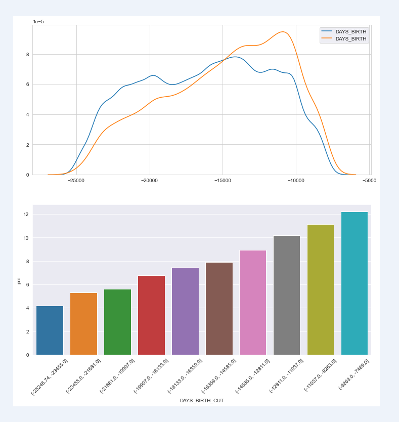
User age distribution: because age is a continuous variable, use and distribution diagram to view user distribution (histogram can also well describe the distribution); Then through the histogram to show the default rate, we can clearly see that the younger the age, the higher the default rate;

chart_fuc(train,"DAYS_BIRTH",con_ornot="continuity",cutn=10)

Default rate of each segment

           DAYS_BIRTH_CUT   sum  count    pro
0  (-25246.74, -23455.0]   503  11977   4.20
1   (-23455.0, -21681.0]  1466  27685   5.30
2   (-21681.0, -19907.0]  1826  32650   5.59
3   (-19907.0, -18133.0]  2278  33544   6.79
4   (-18133.0, -16359.0]  2558  34339   7.45
5   (-16359.0, -14585.0]  3185  40356   7.89
6   (-14585.0, -12811.0]  3737  41746   8.95
7   (-12811.0, -11037.0]  3916  38424  10.19
8    (-11037.0, -9263.0]  3687  33111  11.14
9     (-9263.0, -7489.0]  1669  13679  12.20

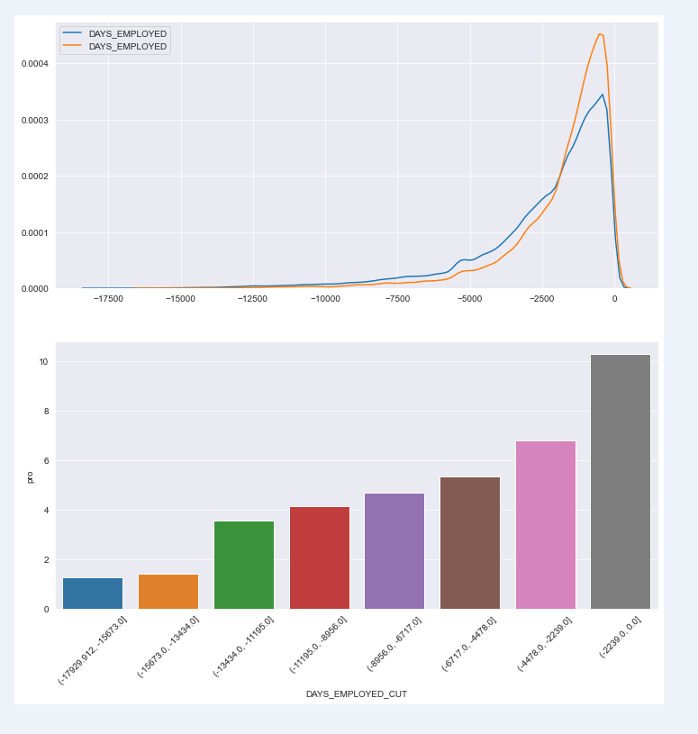
The default distribution of users' employment days is extremely obvious. The fewer employment days, the higher the default rate of users

chart_fuc(train,"DAYS_EMPLOYED",con_ornot="continuity")

Default rate of each segment

         DAYS_EMPLOYED_CUT    sum   count    pro
0  (-17929.912, -15673.0]      1      79   1.27
1    (-15673.0, -13434.0]      8     570   1.40
2    (-13434.0, -11195.0]     72    2028   3.55
3     (-11195.0, -8956.0]    166    4007   4.14
4      (-8956.0, -6717.0]    413    8828   4.68
5      (-6717.0, -4478.0]   1104   20719   5.33
6      (-4478.0, -2239.0]   4181   61310   6.82
7          (-2239.0, 0.0]  15890  154596  10.28

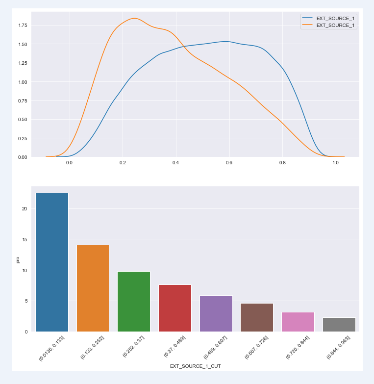
There is a corresponding relationship between external data source standardization score and default rate. The lower the external data source standardization score, the higher the default rate;

chart_fuc(train,"EXT_SOURCE_1",con_ornot="continuity")

Default rate of each segment

   EXT_SOURCE_1_CUT   sum  count    pro
0  (0.0136, 0.133]   978   4344  22.51
1   (0.133, 0.252]  2112  15024  14.06
2    (0.252, 0.37]  2057  21026   9.78
3    (0.37, 0.489]  1778  23240   7.65
4   (0.489, 0.607]  1380  23670   5.83
5   (0.607, 0.726]  1045  22891   4.57
6   (0.726, 0.844]   581  18587   3.13
7   (0.844, 0.963]   123   5351   2.30

In addition, the user's marriage, whether there are children, the number of family members, living area and other factors have an impact on the default rate. You can call chart one by one_ Fuc function to view user distribution map and user default rate distribution map

Characteristic Engineering

"Data and features determine the upper limit of machine learning, while models and algorithms only approach this upper limit". Feature engineering refers to the process of transforming the original data into the training data of the model. Its purpose is to obtain better training data features and make the machine learning model approach this upper limit. Generally speaking, it includes three parts: feature construction, feature extraction and feature selection;
Feature construction refers to manually finding some physical features from the original data.
Feature extraction: principal component analysis, LDA linear discriminant analysis, independent component analysis
Feature selection is to eliminate irrelevant or redundant features, reduce the number of effective features, reduce the time of model training and improve the accuracy of the model.
For Feature Engineering, see: https://www.cnblogs.com/wxquare/p/5484636.html

Combined with business understanding, build features

CREDIT_INCOME_PERCENT: loan amount / customer income, AMT_CREDIT/AMT_INCOME_TOTAL, it is expected that the greater the ratio, the greater the possibility of user default
ANNUITY_INCOME_PERCENT: annual repayment amount of loan / customer income, AMT_ ANNUITY/AMT_ INCOME_ The total logic is consistent with the above
CREDIT_TERM: annual repayment amount of loan / loan amount, repayment cycle of loan, AMT_ANNUITY /AMT_CREDIT, the repayment cycle is a common way of risk management of credit institutions. Theoretically, the customer risk is large, and the credit institutions will shorten the repayment cycle. The distribution map of repayment cycle and default rate should show some information;
DAYS_EMPLOYED_PERCENT: user working time / user age, DAYS_EMPLOYED/DAYS_BIRTH
INCOME_PER_CHILD: customer income / number of children, AMT_INCOME_TOTAL /CNT_CHILDREN, the customer's income is distributed to every child on average. For the same income, if this person has a large family and many children, his burden may be heavy and the possibility of default may be higher
HAS_HOUSE_INFORMATION: Here we design a binary feature according to whether the customer has missing house information. If it is not missing, it is 1 and the missing is 0

train["CREDIT_INCOME_PERCENT"]=(train["AMT_CREDIT"]/train["AMT_INCOME_TOTAL"]).round(2)
train['ANNUITY_INCOME_PERCENT'] = (train['AMT_ANNUITY'] /train['AMT_INCOME_TOTAL']).round(2)
train['CREDIT_TERM'] =(train['AMT_ANNUITY'] /train['AMT_CREDIT']).round(2)
train['DAYS_EMPLOYED_PERCENT'] = (train['DAYS_EMPLOYED'] /train['DAYS_BIRTH']).round(2)
train['INCOME_PER_CHILD'] = (train['AMT_INCOME_TOTAL'] /train['CNT_CHILDREN']).round(2)
train['HAS_HOUSE_INFORMATION'] = train['COMMONAREA_MEDI'].apply(lambda x:1 if x>0 else 0)

Call the chart function defined above to observe the distribution of new features and default rate;

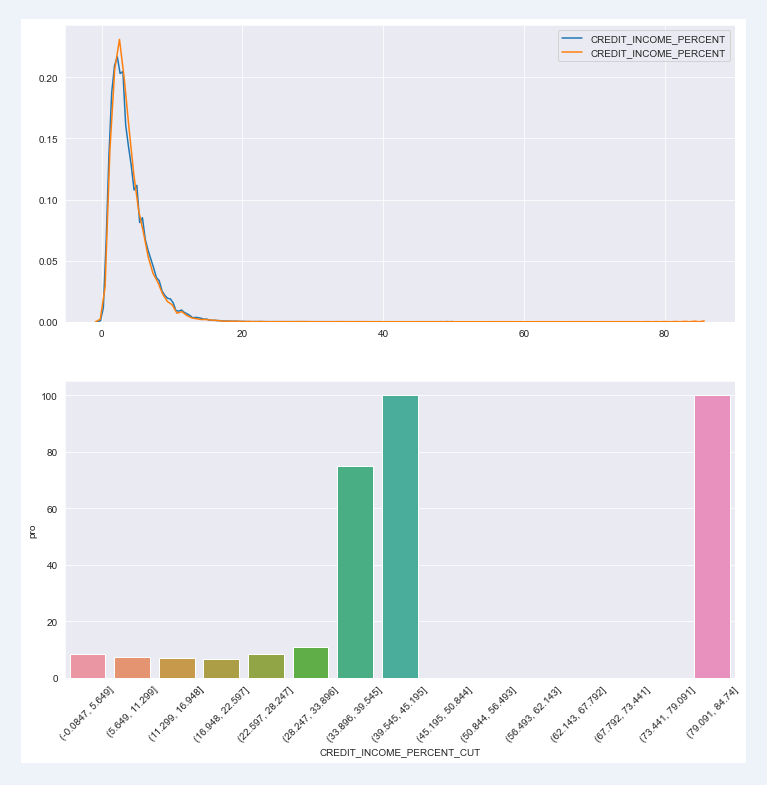
Loan amount / customer income: excluding extreme values and individual cases, the results shown in the distribution map are not quite consistent with our imagination; The question is whether to determine whether the features are invalid or remain and wait for the meeting to test the effect in the model, which is a question worthy of deep thinking and exploration

chart_fuc(train,"CREDIT_INCOME_PERCENT",con_ornot="continuity",cutn=15)

Default rate of each segment

    CREDIT_INCOME_PERCENT_CUT    sum   count     pro
0           (-0.0847, 5.649]  20083  242503    8.28
1            (5.649, 11.299]   4305   58657    7.34
2           (11.299, 16.948]    386    5685    6.79
3           (16.948, 22.597]     35     535    6.54
4           (22.597, 28.247]      8      96    8.33
5           (28.247, 33.896]      3      28   10.71
6           (33.896, 39.545]      3       4   75.00
7           (39.545, 45.195]      1       1  100.00
8           (45.195, 50.844]      0       1    0.00
9           (50.844, 56.493]      0       0     NaN
10          (56.493, 62.143]      0       0     NaN
11          (62.143, 67.792]      0       0     NaN
12          (67.792, 73.441]      0       0     NaN
13          (73.441, 79.091]      0       0     NaN
14           (79.091, 84.74]      1       1  100.00

Whether the applicant has housing information has a significant impact on the default rate. Moreover, users without real estate information account for the majority of the total user group. This is a problem. Whether the target group of the company itself has this feature or the point to be optimized needs to be discussed and analyzed in combination with the actual business

chart_fuc(train,"HAS_HOUSE_INFORMATION")

   HAS_HOUSE_INFORMATION  TARGET_SUM  TARGET_COUNT  Default_Rate
0                      0       18998        223556          8.50
1                      1        5827         83955          6.94

Modeling and prediction

If the model is LGB model, should the specific model be studied by Algorithm Engineers? There is a great God who can give directions to this part; If a person is proficient in the whole model process, including feature engineering and the underlying logic of the model, is he a "successful person"!!!

Differences and relations among lightgbm, xgboost and gbdt https://www.cnblogs.com/mata123/p/7440774.html

from sklearn.model_selection import KFold
from sklearn.metrics import roc_auc_score
from sklearn import preprocessing
import lightgbm as lgb
import gc

Modeling: model training

# The parameters are interpreted as training and test_data is the test set, encoding is the way to convert the classification field into value, one hot or LabelEncoder;
# Cross validation n_folds is the number of layers of training set (divided into training set and verification set)

def model(features, test_features, encoding = 'ohe', n_folds = 5):

    
    # Extract the ID. the ID in the training set and test set has no effect on the feature and needs to be deleted
    train_ids = features['SK_ID_CURR']
    test_ids = test_features['SK_ID_CURR']
    
    # Target of extracting training set: default 0 1;
    labels = features['TARGET']
    
    # Delete the target and ID in the training set to form a new training set (because the training set does not need the target and ID)
    features = features.drop(columns = ['SK_ID_CURR', 'TARGET'])
    test_features = test_features.drop(columns = ['SK_ID_CURR'])
    
    
    # Convert the classification field to the attribute value field One Hot, corresponding to the LabelEncoder below
    if encoding == 'ohe':
        features = pd.get_dummies(features)
        test_features = pd.get_dummies(test_features)
        
        # Aligning the training set requires the field order of the test set, or the alignment feature order. inner indicates the alignment method. Delete the redundant columns (features) between the training set and the test set
        features,test_features = features.align(test_features, join = 'inner', axis = 1)
        
        # No categorical indications to record
        cat_indices = 'auto'
    
    # Assign labels to a 0-n_ Integers between classes-1, standardized. One Hot is horizontal and LabelEncoder is vertical;
    elif encoding == 'le':
        
        # Create LabelEncoder instance object
        le = LabelEncoder()
        
        # An index used to record classification features
        cat_indices = []
        
        # Traverse each column. enumerate means enumerating elements one by one. It returns the elements and their corresponding indexes
        for i, col in enumerate(features):
            if features[col].dtype == 'object':
                # Convert the classification features of training set and test set into integers in the way of LabelEncoder
                features[col] = le.fit_transform(np.array(features[col].astype(str)).reshape((-1,)))
                test_features[col] = le.transform(np.array(test_features[col].astype(str)).reshape((-1,)))

                # Record the classification index, and the results are [3, 4, 5, 11, 12, 13, 14, 15, 28, 32, 40, 86, 87, 89, 90]
                cat_indices.append(i)
    
    # One of the conversion methods of One Hot or LabelEncoder must be selected
    else:
        raise ValueError("Encoding must be either 'ohe' or 'le'")
        
    print('Training Data Shape: ', features.shape)
    print('Testing Data Shape: ', test_features.shape)
    
    # Record feature name, i.e. column name
    feature_names = list(features.columns)
    
    # Convert DataFrame to tuple
    features = np.array(features)
    test_features = np.array(test_features)
    
    # Create kfold instance object to form training set and verification set, n_folds is the parameter defined by the model function
    k_fold = KFold(n_splits = n_folds, shuffle = True, random_state = 50)
    
    # 0 tuple used to record feature importance
    feature_importance_values = np.zeros(len(feature_names))
    
    # 0 tuple used to record test set prediction results
    test_predictions = np.zeros(test_features.shape[0])
    
    # 0 tuple used to record the result of training set
    out_of_fold = np.zeros(features.shape[0])
    
    # Lists for recording validation and training scores
    valid_scores = []
    train_scores = []
    
    # The training set is divided into new training set and verification set through kfold, and the training model is established
    for train_indices, valid_indices in k_fold.split(features):
        
        # Default label corresponding to the new training set
        train_features, train_labels = features[train_indices], labels[train_indices]
        # Validation set and default label corresponding to validation set
        valid_features, valid_labels = features[valid_indices], labels[valid_indices]
        
        # Instantiated LGB model
        model = lgb.LGBMClassifier(n_estimators=1000, objective = 'binary', 
                                   class_weight = 'balanced', learning_rate = 0.05, 
                                   reg_alpha = 0.1, reg_lambda = 0.1, 
                                   subsample = 0.8, n_jobs = -1, random_state = 50)
        
        # Training model
        model.fit(train_features, train_labels, eval_metric = 'auc',
                  eval_set = [(valid_features, valid_labels), (train_features, train_labels)],
                  eval_names = ['valid', 'train'], categorical_feature = cat_indices,
                  early_stopping_rounds = 100, verbose = 200)
        
        # Record the best iteration
        best_iteration = model.best_iteration_
        
        # Importance of recording characteristics
        feature_importance_values += model.feature_importances_ / k_fold.n_splits
        
        # Training set prediction
        test_predictions += model.predict_proba(test_features, num_iteration = best_iteration)[:, 1] / k_fold.n_splits
        
        #  Record the prediction of the validation set
        out_of_fold[valid_indices] = model.predict_proba(valid_features, num_iteration = best_iteration)[:, 1]
        
        # Record high score
        valid_score = model.best_score_['valid']['auc']
        train_score = model.best_score_['train']['auc']
        
        valid_scores.append(valid_score)
        train_scores.append(train_score)
        
        # Clear memory
        gc.enable()
        del model, train_features, valid_features
        gc.collect()
        
    # Record the prediction results of the training set, DataFrame structure
    submission = pd.DataFrame({'SK_ID_CURR': test_ids, 'TARGET': test_predictions})
    
    # Record feature importance, DataFrame structure
    feature_importances = pd.DataFrame({'feature': feature_names, 'importance': feature_importance_values})
    
    # Overall verification score: roc curve area
    valid_auc = roc_auc_score(labels, out_of_fold)
    
    # Verification set score and training set score
    valid_scores.append(valid_auc)
    train_scores.append(np.mean(train_scores))
    
    # Record all validation sets and overall scores
    fold_names = list(range(n_folds))
    fold_names.append('overall')
    
    # Record all validation sets and overall scores, DataFrame structure
    metrics = pd.DataFrame({'fold': fold_names,
                            'train': train_scores,
                            'valid': valid_scores}) 
    
    # Returns the prediction result, feature importance and model score of the training set
    return submission, feature_importances, metrics

Model ROC score

submission, fi, metrics = model(train,test)
print("=="*50)
print("Model ROC score\n",metrics)

Training Data Shape:  (307511, 241)
Testing Data Shape:  (48744, 241)
Training until validation scores don't improve for 100 rounds
[200]	train's auc: 0.7986	train's binary_logloss: 0.547763	valid's auc: 0.755506	valid's binary_logloss: 0.563315
[400]	train's auc: 0.828273	train's binary_logloss: 0.518238	valid's auc: 0.755427	valid's binary_logloss: 0.545289
Early stopping, best iteration is:
[355]	train's auc: 0.822307	train's binary_logloss: 0.524257	valid's auc: 0.755636	valid's binary_logloss: 0.548978
Training until validation scores don't improve for 100 rounds
[200]	train's auc: 0.798864	train's binary_logloss: 0.547653	valid's auc: 0.758325	valid's binary_logloss: 0.563454
Early stopping, best iteration is:
[245]	train's auc: 0.806436	train's binary_logloss: 0.540255	valid's auc: 0.758595	valid's binary_logloss: 0.558896
Training until validation scores don't improve for 100 rounds
[200]	train's auc: 0.797785	train's binary_logloss: 0.549132	valid's auc: 0.76297	valid's binary_logloss: 0.56397
Early stopping, best iteration is:
[244]	train's auc: 0.805083	train's binary_logloss: 0.542037	valid's auc: 0.763298	valid's binary_logloss: 0.559489
Training until validation scores don't improve for 100 rounds
[200]	train's auc: 0.798991	train's binary_logloss: 0.547787	valid's auc: 0.758187	valid's binary_logloss: 0.562107
Early stopping, best iteration is:
[245]	train's auc: 0.806411	train's binary_logloss: 0.540463	valid's auc: 0.758239	valid's binary_logloss: 0.557764
Training until validation scores don't improve for 100 rounds
[200]	train's auc: 0.798045	train's binary_logloss: 0.548459	valid's auc: 0.757937	valid's binary_logloss: 0.564587
[400]	train's auc: 0.828024	train's binary_logloss: 0.518946	valid's auc: 0.757796	valid's binary_logloss: 0.54673
Early stopping, best iteration is:
[315]	train's auc: 0.816215	train's binary_logloss: 0.53072	valid's auc: 0.75831	valid's binary_logloss: 0.553896
====================================================================================================
Model ROC score
       fold     train     valid
0        0  0.822307  0.755636
1        1  0.806436  0.758595
2        2  0.805083  0.763298
3        3  0.806411  0.758239
4        4  0.816215  0.758310
5  overall  0.811290  0.758783

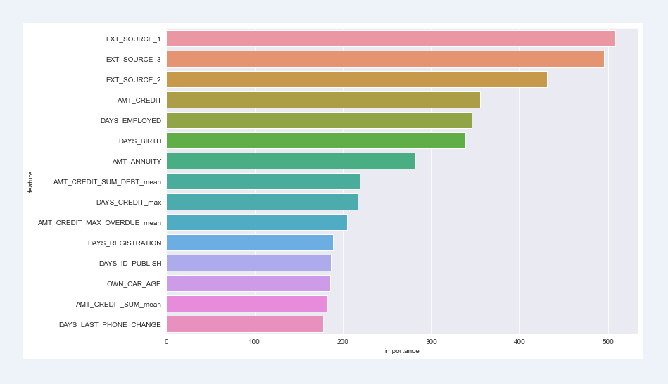
Feature importance top15

It can be seen that the impact of external data on default is more prominent. In other words, the prediction data given by the outside is more referential. In addition to external data, the user's age, working years, income, loan amount, car years, and population distribution in the customer's living area also have a great impact on the breach of contract

fi15=fi.sort_values("importance",ascending=False).head(15)
plt.figure(figsize=(12,8))
sns.set_style("darkgrid")
sns.barplot(x="importance",y="feature",data=fi15,orient="h")

<matplotlib.axes._subplots.AxesSubplot at 0x25887eb0>

There are also some features that have a weak impact on user breach of contract, such as the type of customer work organization and the situation of accompanying personnel during application, which may be inconsistent with our understanding in fact. It is also possible that the situation abroad is different from that at home. In short, it needs to be comprehensively analyzed in combination with the actual business products. The impact of a feature at the moment on default does not explain the future. Therefore, if you want to completely delete the data acquisition of a feature, you still need to make a careful decision;

fil15=fi.sort_values("importance",ascending=True).head(25)
fil15

	feature	importance
121	NAME_INCOME_TYPE_Pensioner	0.0
185	ORGANIZATION_TYPE_Industry: type 13	0.0
190	ORGANIZATION_TYPE_Industry: type 6	0.0
192	ORGANIZATION_TYPE_Industry: type 8	0.0
173	ORGANIZATION_TYPE_Cleaning	0.0
199	ORGANIZATION_TYPE_Mobile	0.0
204	ORGANIZATION_TYPE_Religion	0.0
78	FLAG_DOCUMENT_2	0.0
80	FLAG_DOCUMENT_4	0.0
83	FLAG_DOCUMENT_7	0.0
216	ORGANIZATION_TYPE_Trade: type 5	0.0
86	FLAG_DOCUMENT_10	0.0
88	FLAG_DOCUMENT_12	0.0
96	FLAG_DOCUMENT_20	0.0
224	ORGANIZATION_TYPE_XNA	0.0
105	NAME_CONTRACT_TYPE_Revolving loans	0.0
182	ORGANIZATION_TYPE_Industry: type 10	0.0
14	FLAG_CONT_MOBILE	0.0
109	FLAG_OWN_CAR_Y	0.0
119	NAME_INCOME_TYPE_Businessman	0.0
12	FLAG_EMP_PHONE	0.0
11	FLAG_MOBIL	0.0
123	NAME_INCOME_TYPE_Student	0.0
114	NAME_TYPE_SUITE_Group of people	0.0
97	FLAG_DOCUMENT_21	0.2

So far, even if a complete model prediction process is over, the total score of the model is within the acceptable range, which is a reference for users' review. The following is to extract new features from auxiliary set data to improve the model and improve the effect of the model.

Other dataset information

bureau=pd.read_csv(r"C:\Users\TP\Desktop\myself\Loan risk\Credit risk data set\bureau.csv")

Discrete variable (characterized by discrete type)

There are various ways to convert discrete variables into eigenvalues, which can be determined according to the model score in combination with the actual business or through the training model. For example, credit in bureau of credit information_ Active users may have multiple credit cards with different statuses, 'Closed', 'active', 'Sold', 'Bad debt'. Treatment method 1: we can only keep the state with the highest risk and delete others. For example, if the user has both 'active' and 'Bad debt', we can keep 'Bad debt' and delete 'active'; Processing method 2: we use the statistical function count to record the number of each state to form a new feature field; Although many companies adopt the first processing method, here we adopt the second one for convenience and define a unified discrete variable processing function;

#Definition of discrete variable processing function
def dispersed_featrue(data,featrue):
    dg=data.groupby(["SK_ID_CURR",featrue])[featrue].count()
    
    # Fill null values with 0
    dc=dg.unstack(fill_value=0)
    
    # New field naming
    col=[]
    for i in  np.arange(len(dc.columns)):
        new_col=featrue + "_" + dc.columns[i]
        col.append(new_col)
    dc.columns=col
    dc.reset_index(inplace=True)
    return dc
#There is another convenient method: get_dummies, no more details

Continuous variable (characterized by continuous type)

Continuous variables can be described by one or more of the mean, quantile, mode, variance, etc. in the statistical value

# Definition of continuous variable processing function
def continuos_featrue(data,featrue,statistics):
    df=data.groupby("SK_ID_CURR")[featrue].agg(statistics)
    df.reset_index(inplace=True)
    
    # New field naming
    col=["SK_ID_CURR"]
    for i in  np.arange(len(df.columns)-1):
        new_col=featrue + "_" + df.columns[i+1]
        col.append(new_col)
    df.columns=col
    return df

Convert the discrete variables and continuous variables in the credit report into analytical features with the above defined functions;
Discrete variable: CREDIT_ACTIVE (credit report status), CREDIT_CURRENCY, CREDIT_TYPE (loan type)
Continuous variable: DAYS_CREDIT (how many days before the current application, the customer has applied for credit)_ DAY_ Overdue (when the customer in the sample applies for a loan, how many days will the previously applied loan expire), AMT_ CREDIT_ MAX_ Overdrue (the highest amount of customer loan so far), CNT_CREDIT_PROLONG (times of deferred repayment in the customer's previous loan), AMT_CREDIT_SUM (loan limit of credit institution), AMT_CREDIT_SUM_DEBT (current debt of credit institutions), AMT_CREDIT_SUM_LIMIT (current credit card limit), AMT_CREDIT_SUM_ Overdrue (overdue amount of loans from credit institutions), AMT_ANNUITY (annual loan limit of credit institution)

# discrete variable 
ca=dispersed_featrue(bureau,"CREDIT_ACTIVE")
cc=dispersed_featrue(bureau,"CREDIT_CURRENCY")
ct=dispersed_featrue(bureau,"CREDIT_TYPE")

#continuous variable 
dc=continuos_featrue(bureau,"DAYS_CREDIT",["mean","max"])
cdo=continuos_featrue(bureau,"CREDIT_DAY_OVERDUE",["mean","max"])
acmo=continuos_featrue(bureau,"AMT_CREDIT_MAX_OVERDUE",["mean","max"])
ccp=continuos_featrue(bureau,"CNT_CREDIT_PROLONG",["mean","max"])
acs=continuos_featrue(bureau,"AMT_CREDIT_SUM",["mean","max","sum"])
acd=continuos_featrue(bureau,"AMT_CREDIT_SUM_DEBT",["mean","max","sum"])
acsl=continuos_featrue(bureau,"AMT_CREDIT_SUM_LIMIT",["mean","max","sum"])
acso=continuos_featrue(bureau,"AMT_CREDIT_SUM_OVERDUE",["mean","max","sum"])
aa=continuos_featrue(bureau,"AMT_ANNUITY",["mean","max","sum"])

Connect to the training set to form a new training set

col=[ca,cc,ct,dc,cdo,acmo,ccp,acs,acd,acsl,acso,aa]
for i in np.arange(len(col)):
    train=pd.merge(train,col[i],how="inner",on="SK_ID_CURR")
    test=pd.merge(test,col[i],how="inner",on="SK_ID_CURR")
train.head()

	SK_ID_CURR	TARGET	NAME_CONTRACT_TYPE	CODE_GENDER	FLAG_OWN_CAR	FLAG_OWN_REALTY	AMT_INCOME_TOTAL	AMT_CREDIT	AMT_ANNUITY	...	AMT_CREDIT_SUM_DEBT_sum	AMT_CREDIT_SUM_LIMIT_mean	AMT_CREDIT_SUM_LIMIT_max	AMT_CREDIT_SUM_LIMIT_sum	AMT_ANNUITY_mean	AMT_ANNUITY_max
0	100002	1	Cash loans	M	N	Y	202500.0	406597.5	24700.5	...	245781.0	7997.14125	31988.565	31988.565	0.0	0.0
1	100003	0	Cash loans	F	N	N	270000.0	1293502.5	35698.5	...	0.0	202500.00000	810000.000	810000.000	NaN	NaN
2	100004	0	Revolving loans	M	Y	Y	67500.0	135000.0	6750.0	...	0.0	0.00000	0.000	0.000	NaN	NaN
3	100007	0	Cash loans	M	N	Y	121500.0	513000.0	21865.5	...	0.0	0.00000	0.000	0.000	NaN	NaN
4	100008	0	Cash loans	M	N	Y	99000.0	490495.5	27517.5	...	240057.0	0.00000	0.000	0.000	NaN	NaN

5 rows × 174 columns

So far, a new training set has been formed combined with auxiliary data; According to the actual situation, there will be more new features. The data determines the upper limit of the model, and feature construction requires considerable business understanding, which is a fine activity. Feature construction is not explored here

As for the selection of features, some features with collinearity are excluded to improve the effect of the model. The correlation coefficient between variables can be calculated to quickly remove some variables with high correlation. Here, a threshold value of 0.8 can be defined, that is, remove one of the variables in each pair of variables with correlation greater than 0.8;
In addition, variables insensitive to the target response will also affect the accuracy of the model. These variables can be deleted according to the correlation coefficient or the importance of model characteristics. The reason is the same as above and will not be repeated;

df=train.drop(columns=["SK_ID_CURR","TARGET"])
df=df.corr()

# Define an empty list to record the features that need to be deleted because the correlation is greater than 0.8
ft=[] 
for col in df:
     if col not in ft:
            d=df.index[df[col] >0.8].to_list()
            if col in d :
                d.remove(col)
                ft.extend(d)
                
# Delete variables whose correlation is greater than the threshold
train.drop(columns=ft,inplace=True)

train.head()

	SK_ID_CURR	TARGET	NAME_CONTRACT_TYPE	CODE_GENDER	FLAG_OWN_CAR	FLAG_OWN_REALTY	AMT_INCOME_TOTAL	AMT_CREDIT	AMT_ANNUITY	...	AMT_CREDIT_SUM_mean	AMT_CREDIT_SUM_sum	AMT_CREDIT_SUM_DEBT_mean	AMT_CREDIT_SUM_DEBT_max	AMT_CREDIT_SUM_LIMIT_mean	AMT_CREDIT_SUM_LIMIT_max	AMT_ANNUITY_mean	AMT_ANNUITY_max
0	100002	1	Cash loans	M	N	Y	202500.0	406597.5	24700.5	...	108131.945625	865055.565	49156.2	245781.0	7997.14125	31988.565	0.0	0.0
1	100003	0	Cash loans	F	N	N	270000.0	1293502.5	35698.5	...	254350.125000	1017400.500	0.0	0.0	202500.00000	810000.000	NaN	NaN
2	100004	0	Revolving loans	M	Y	Y	67500.0	135000.0	6750.0	...	94518.900000	189037.800	0.0	0.0	0.00000	0.000	NaN	NaN
3	100007	0	Cash loans	M	N	Y	121500.0	513000.0	21865.5	...	146250.000000	146250.000	0.0	0.0	0.00000	0.000	NaN	NaN
4	100008	0	Cash loans	M	N	Y	99000.0	490495.5	27517.5	...	156148.500000	468445.500	80019.0	240057.0	0.00000	0.000	NaN	NaN

5 rows × 126 columns

Retraining model

submission, fi, metrics = model(train,test)
print("=="*50)
print("Model ROC score\n",metrics)

Training Data Shape:  (263491, 239)
Testing Data Shape:  (42320, 239)
Training until validation scores don't improve for 100 rounds
[200]	train's auc: 0.814678	train's binary_logloss: 0.532306	valid's auc: 0.766264	valid's binary_logloss: 0.5511
Early stopping, best iteration is:
[249]	train's auc: 0.823937	train's binary_logloss: 0.522804	valid's auc: 0.766576	valid's binary_logloss: 0.545026
Training until validation scores don't improve for 100 rounds
[200]	train's auc: 0.814559	train's binary_logloss: 0.532478	valid's auc: 0.767164	valid's binary_logloss: 0.551391
Early stopping, best iteration is:
[283]	train's auc: 0.830264	train's binary_logloss: 0.516345	valid's auc: 0.767488	valid's binary_logloss: 0.541334
Training until validation scores don't improve for 100 rounds
[200]	train's auc: 0.814355	train's binary_logloss: 0.533096	valid's auc: 0.771143	valid's binary_logloss: 0.549807
Early stopping, best iteration is:
[284]	train's auc: 0.830247	train's binary_logloss: 0.516858	valid's auc: 0.771516	valid's binary_logloss: 0.539648
Training until validation scores don't improve for 100 rounds
[200]	train's auc: 0.815806	train's binary_logloss: 0.530951	valid's auc: 0.75585	valid's binary_logloss: 0.550364
Early stopping, best iteration is:
[297]	train's auc: 0.833183	train's binary_logloss: 0.512621	valid's auc: 0.756601	valid's binary_logloss: 0.538989
Training until validation scores don't improve for 100 rounds
[200]	train's auc: 0.813839	train's binary_logloss: 0.532965	valid's auc: 0.767956	valid's binary_logloss: 0.548167
Early stopping, best iteration is:
[210]	train's auc: 0.81593	train's binary_logloss: 0.530808	valid's auc: 0.768212	valid's binary_logloss: 0.546807
====================================================================================================
Model ROC score
       fold     train     valid
0        0  0.823937  0.766576
1        1  0.830264  0.767488
2        2  0.830247  0.771516
3        3  0.833183  0.756601
4        4  0.815930  0.768212
5  overall  0.826712  0.765973

fi15=fi.sort_values("importance",ascending=False).head(15)
plt.figure(figsize=(12,8))
sns.set_style("darkgrid")
sns.barplot(x="importance",y="feature",data=fi15,orient="h")

<matplotlib.axes._subplots.AxesSubplot at 0x2b2f4790>

Adding a new training set composed of new features filtered by the auxiliary training set to train the model, the result is better than the original training set training model. It can also be seen from the feature importance that some features constructed through the auxiliary training set are also of high importance and perform well

So far, the whole model building process has ended; Model building is a continuous iterative process, including feature engineering optimization, new data collection, algorithm optimization and so on.

Keywords: Python Data Analysis

Added by Darhazer on Tue, 01 Feb 2022 16:10:52 +0200

Programming VIP