**

1 - Packages (import package, load dataset)

1.1 import package

The Python packages used include:
◎ numpy is a basic package for scientific computing using Python.
◎ h5py Python provides an interface for reading HDF5 binary data format files. This training and test picture set is stored in HDF5.
◎ matplotlib is a famous drawing library in Python.
◎ PIL (Python Image Library) provides image processing functions for Python.
◎ scipy is based on NumPy to expand the library of advanced mathematics, signal processing, optimization, statistics and many other scientific tasks.
Programming implementation of import package:

import numpy as np                   #numpy is a basic package for scientific computing using Python.
import matplotlib.pyplot as plt      #It is a famous drawing library in Python.
import h5py                          #Based on NumPy to do advanced mathematics, signal processing, optimization, statistics and many other scientific tasks.
import scipy                         ##ython provides an interface to read HDF5 binary data format files. This training and test picture set is stored in HDF5.
from PIL import Image                #(Python Image Library) provides image processing functions for Python
from scipy import ndimage
from lr_utils import load_dataset    # Used to import datasets
#%matplotlib inline   #Set matplotlib to display pictures in rows

1.2 loading data package

New file lr_utils.py
#Warm tip: if the job runs locally, the code of the dataset is saved in lr_utils.py file and save it in a folder with the current project
Programming implementation of loading data set:

2 - Overview of the Problem set

2.1 importing data

Programming implementation:

import numpy as np
import h5py
"""
    train_set_x_orig : The image data in the training set is saved (there are 209 64 images in this training set) x64 Image).
    train_set_y_orig : What is saved is the classification value corresponding to the image of the training set ([0 | 1]，0 Means not a cat, 1 means a cat).
    test_set_x_orig : The image data in the test set is saved (there are 50 64 images in this training set) x64 Image).
    test_set_y_orig :  What is saved is the classification value corresponding to the image of the test set ([0 | 1]，0 Means not a cat, 1 means a cat).
    classes :  Saved in bytes Type saves two string data, the data is:[b'non-cat' b'cat']. 
"""
#HDF5 File is a container for storing dataset and group data objects, and its operation is similar to the File operation of python standard; the File instance object itself is a group, named / and is the entry for traversing the File.
#H5py.file (file name, which can be byte string or unicode string, 'mode')  
def load_dataset():
    train_dataset = h5py.File('datasets/train_catvnoncat.h5', "r")
    train_set_x_orig = np.array(train_dataset["train_set_x"][209]) 
    train_set_y_orig = np.array(train_dataset["train_set_y"][:]) 

    test_dataset = h5py.File('datasets/test_catvnoncat.h5', "r")
    test_set_x_orig = np.array(test_dataset["test_set_x"][:]) 
    test_set_y_orig = np.array(test_dataset["test_set_y"][:]) 

    classes = np.array(test_dataset["list_classes"][:])
    
    train_set_y_orig = train_set_y_orig.reshape((1, train_set_y_orig.shape[0]))
    test_set_y_orig = test_set_y_orig.reshape((1, test_set_y_orig.shape[0]))
    
    return train_set_x_orig, train_set_y_orig, test_set_x_orig, test_set_y_orig, classes

2.2 test data programming:

#Test data

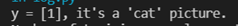
index = 25 #Number of tags
plt.imshow(train_set_x_orig[index])
print ("y = " + str(train_set_y_orig[:,index]) + ", it's a '" + classes[np.squeeze(test_set_y_orig[:,index])].decode("utf-8") +  "' picture.")

Programming output:

2.3 calculate the size of training set, test set and image

Programming implementation:

#Calculate the size of training set, test set and image
m_train = train_set_y_orig.shape[1]
m_test = test_set_y_orig.shape[1]
num_px = train_set_x_orig.shape[1]
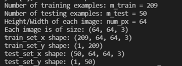
print ("Number of training examples: m_train = " + str(m_train))
print ("Number of testing examples: m_test = " + str(m_test))
print ("Height/Width of each image: num_px = " + str(num_px))
print ("Each image is of size: (" + str(num_px) + ", " + str(num_px) + ", 3)")
print ("train_set_x shape: " + str(train_set_x_orig.shape))
print ("train_set_y shape: " + str(train_set_y_orig.shape))
print ("test_set_x shape: " + str(test_set_x_orig.shape))
print ("test_set_y shape: " + str(test_set_y_orig.shape))

Programming results:

2.4 conversion matrix

The whole training set is transformed into a matrix, including num_pxnum_py3 rows and m_train columns.
Where X_flatten = X.reshape(X.shape[0], -1).T can: convert a matrix with dimension (a,b,c,d) into a matrix with dimension (b * c * d, a).
Programming implementation:
#Transformation matrix
#The whole training set is transformed into a matrix, including num_pxnum_py3 rows and m_train columns

train_set_x_flatten = train_set_x_orig.reshape(train_set_x_orig.shape[0],-1).T
test_set_x_flatten = test_set_x_orig.reshape(test_set_x_orig.shape[0], -1).T

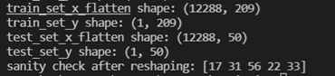
print ("train_set_x_flatten shape: " + str(train_set_x_flatten.shape))
print ("train_set_y shape: " + str(train_set_y_orig.shape))
print ("test_set_x_flatten shape: " + str(test_set_x_flatten.shape))
print ("test_set_y shape: " + str(test_set_y_orig.shape))
print ("sanity check after reshaping: " + str(train_set_x_flatten[0:5,0]))

Programming results:

2.5 preprocessing data (decentralization)

In order to represent an image (RGB), each pixel must be specified. In fact, the pixel value is a vector of three numbers (0-255))
Usually, the preprocessing work of machine learning is to decentralize and standardize your data set, (x - mean) / standard deviation. However, for image data set, it is easier and more efficient to divide each row of the data set by 255 (the pixel channel of the maximum value)
Programming implementation:

#Decentralization
train_set_x = train_set_x_flatten / 255
test_set_x = test_set_x_flatten / 255

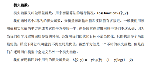
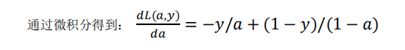
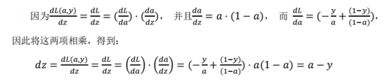
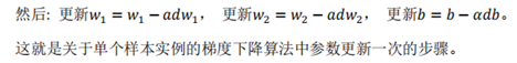
Cost function and cost knowledge supplement:

3 - Building the parts of our algorithm

Main steps of building a neural network:

1. Define the structure of the model (for example, the number of input features)
2. Initialize the parameters of the model
3. Cyclic operation
   Calculate the current loss value (forward propagation)
   Calculate the current gradient value (back propagation)
   Updating parameters, gradient descent algorithm

3.1 - sigmod() function implementation

To implement the sigmod() function, you need to calculate sigmoid(wTx+b) to predict
Programming implementation:

#sigmoid() function implementation
def sigmoid(z):
    """
    Compute the sigmoid of z

    Arguments:
    x -- A scalar or numpy array of any size.

    Return:
    s -- sigmoid(z)
    """
    s = 1 / (1 + np.exp(-z))
return s
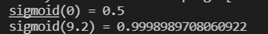
print ("sigmoid(0) = " + str(sigmoid(0)))
print ("sigmoid(9.2) = " + str(sigmoid(9.2)))

Programming results:

3.2 - initialization parameters (w, b)

Implement parameter initialization below. You have to initialize w to a zero vector. Use np.zeros()
Programming implementation:

# Initialization parameters (W, b)
def initialize_with_zeros(dim):
    """
    This function creates a vector of zeros of shape (dim, 1) for w and initializes b to 0.
    
    Argument:
    dim -- size of the w vector we want (or number of parameters in this case)
    
    Returns:
    w -- initialized vector of shape (dim, 1)
    b -- initialized scalar (corresponds to the bias)
    """
    w = np.zeros(shape=(dim, 1))    # Vector initialized w to (dim row, 1 column)
    b = 0
    assert(w,shape == (dim, 1))   # Judge whether the shape of w is (dim, 1). If not, terminate the program
    assert(isinstance(b, float) or isinstance(b, int))   # Determine whether b is of float or int type
    
    return w, b
w,b = initialize_with_zeros(5)
print("w=", w)
print("b=", b)

Programming results:

3.3 - forward and backward propagation
Now that your parameters have been initialized, you can carry out forward propagation and backward propagation steps to learn parameters.
Implement a function ropagate() to calculate the cost function and its gradient
Programming implementation:

# Forward propagation and backward propagation
def propagate(w, b, X, Y):
    """
    Implement the cost function and its gradient for the propagation explained above

    Arguments:
    w -- weights, a numpy array of size (num_px * num_px * 3, 1)
    b -- bias, a scalar
    X -- data of size (num_px * num_px * 3, number of examples)
    Y -- true "label" vector (containing 0 if non-cat, 1 if cat) of size (1, number of examples)

    Return:
    cost -- negative log-likelihood cost for logistic regression
    dw -- gradient of the loss with respect to w, thus same shape as w
    db -- gradient of the loss with respect to b, thus same shape as b
    
    Tips:
    - Write your code step by step for the propagation
    """
    m = X.shape[1]      #Number of samples

    # Forward propagation 
    A = sigmoid(np.dot(w.T, X) + b) # The dimension for calculating activation, a is (m, m)
    cost = (- 1 / m) * np.sum(Y * np.log(A) + (1 - Y) * (np.log(1 - A)))  # Calculate cost; Y == yhat(1, m)
    # Backward propagation 
    dw = (1 / m) * np.dot(X, (A - Y).T) # Calculate the derivative of w
    db = (1 / m) * np.sum(A - Y)          # Calculate the derivative of b

    assert(dw.shape == w.shape)          # Reduce bug s
    assert(db.dtype == float)            # db is a value
    cost = np.squeeze(cost)              # Compress the dimension (delete the one-dimensional entry from the shape of the array, that is, remove the dimension with 1 in the shape), and ensure that cost is the value
    assert(cost.shape == ())
    
    grads = {"dw": dw,
             "db": db}
    
    return grads, cost
w, b, X, Y = np.array([[1], [2]]), 2, np.array([[1,2], [3,4]]), np.array([[1, 0]])
grads, cost = propagate(w, b, X, Y) 
print ("dw = " + str(grads["dw"]))  
print ("db = " + str(grads["db"]))  
print ("cost = " + str(cost))

Programming results:

3.4 optimization

Your parameters have been initialized.
It has been possible to calculate a cost function and its gradient.
Now you need to update the parameters with the gradient descent algorithm.
Write the optimization function. The goal is to learn the parameters w and b by minimizing the cost function J θ， Update rule is θ=θ– α d θ，α Is learning rate)
Programming implementation:

#Optimization
def optimize(w, b, X, Y, num_iterations, learning_rate, print_cost = False):
    """
    This function optimizes w and b by running a gradient descent algorithm

    Arguments:
    w -- weights, a numpy array of size (num_px * num_px * 3, 1)
    b -- bias, a scalar
    X -- data of shape (num_px * num_px * 3, number of examples)
    Y -- true "label" vector (containing 0 if non-cat, 1 if cat), of shape (1, number of examples)
    num_iterations -- number of iterations of the optimization loop  Number of iterations of the optimization cycle
    learning_rate -- learning rate of the gradient descent update rule
    print_cost -- True to print the loss every 100 steps 
    
    Returns:
    params -- Include weight w And deviation b Dictionary of
    grads -- The dictionary contains the gradient of the weight and the deviation from the cost function
    costs -- A list of all costs calculated during the optimization process, which will be used to draw the learning curve.
    
    Tips :
    You basically need to write down two steps and iterate over them:
        1)Calculate the cost and gradient of the current parameter. Use propagation(). 
        2)yes w and b Update parameters using gradient descent rules.
    """
    costs = []
 
    for i in range(num_iterations):
    
        # Cost and gradient calculation     
        grads, cost = propagate(w, b, X, Y)     
        # Retrieve derivatives from grads
        dw = grads["dw"]
        db = grads["db"]

        # update rule
        w = w - learning_rate * dw  # need to broadcast
        b = b - learning_rate * db      
   
        # Record the costs
        if i % 100 == 0:
            costs.append(cost)
        
        # Print the cost every 100 training examples
        if print_cost and i % 100 == 0:
            print ("Cost after iteration %i: %f" % (i, cost))
    
    # Record the iterated parameters (w, b)
    params = {"w": w,
              "b": b}
    
    # Record the current derivative (dw, db) to continue the iteration next time
    grads = {"dw": dw,
             "db": db}
    
    return params, grads, costs
params, grads, costs = optimize(w, b, X, Y, num_iterations= 200, learning_rate = 0.009, print_cost = True)
print ("w = " + str(params["w"]))
print ("b = " + str(params["b"]))
print ("dw = " + str(grads["dw"]))
print ("db = " + str(grads["db"]))

Programming results:

3.5 prediction function

The previous function will output the learned parameters (w, b). We can use w and B to predict the label of dataset x and implement the predict() function. There are two steps to calculate the prediction:

1. Calculate Y_hat = A = sigmod(w.T X + b)
2. Convert a to 0 (if activation < = 0.5) or 1 (if activation > 0.5) and store the predicted value in the vector Y_prediction. If you want, you can use if/else in the for loop (although there is a way to vectorize it)
   Programming implementation:

#Prediction function
#1. Calculate Y_hat = A = sigmod(w.T X + b)
#2. Convert a to 0 (if activation < = 0.5) or 1 (if activation > 0.5), and store the predicted value in vector y_ In prediction
def predict(w, b, X):
    '''
    Predict whether the label is 0 or 1 using learned logistic regression parameters (w, b)
    Arguments:
    w -- weights, a numpy array of size (num_px * num_px * 3, 1)
    b -- bias, a scalar
    X -- data of size (num_px * num_px * 3, number of examples)
    Returns:
    Y_prediction -- a numpy array (vector) containing all predictions (0/1) for the examples in X
    '''
    m = X.shape[1]
    Y_prediction = np.zeros((1, m))
    w = w.reshape(X.shape[0], 1)
    
    # Calculate vector A and predict the probability of A cat in the picture
    A = sigmoid(np.dot(w.T, X) + b)   
    for i in range(A.shape[1]):
        # Convert probability a[0,i] to actual prediction p[0,i]
        Y_prediction[0, i] = 1 if A[0, i] > 0.5 else 0
    
    assert(Y_prediction.shape == (1, m))
    
    return Y_prediction
print("predictions = " + str(predict(w, b, X)))

Programming results:

4 - merge all functions in one model()

You will see how to build the entire model by combining all the builds (the functions implemented in the previous section) in the correct order.
Steps:
Y_prediction: you make predictions on the test set
Y_prediction_train: your prediction on the training set
w. Costs, grads: output of optimize()
Programming implementation:

# Merge all functions in one model()
def model(X_train, Y_train, X_test, Y_test, num_iterations=2000, learning_rate=0.5, print_cost=False):
    """
    Builds the logistic regression model by calling the function you've implemented previously
    
    Arguments:
    X_train -- Training set training set represented by a numpy array of shape (num_px * num_px * 3, m_train)
    Y_train -- Training label training labels represented by a numpy array (vector) of shape (1, m_train)
    X_test -- test set represented by a numpy array of shape (num_px * num_px * 3, m_test)
    Y_test -- test labels represented by a numpy array (vector) of shape (1, m_test)
    num_iterations -- hyperparameter representing the number of iterations to optimize the parameters
    learning_rate -- hyperparameter representing the learning rate used in the update rule of optimize()
    print_cost -- Set to true to print the cost every 100 iterations
    
    Returns:
    d -- dictionary containing information about the model.A dictionary that contains information about the model
    """
    # initialize parameters with zeros
    w, b = initialize_with_zeros(X_train.shape[0])         # num_px*num_px*3

    # Gradient descent (gradient descent update parameter for forward propagation and backward propagation at the same time)
    parameters, grads, costs = optimize(w, b, X_train, Y_train, num_iterations, learning_rate, print_cost)
    
    # Retrieve parameters w and b from dictionary "parameters"
    w = parameters["w"]
    b = parameters["b"]
    
    # Predict test/train set examples
    Y_prediction_train = predict(w, b, X_train)
    Y_prediction_test = predict(w, b, X_test)

    # Print train/test Errors: (100 - mean(abs(Y_hat - Y))*100)
    print("train accuracy: {} %".format(100 - np.mean(np.abs(Y_prediction_train - Y_train)) * 100))
    print("test accuracy: {} %".format(100 - np.mean(np.abs(Y_prediction_test - Y_test)) * 100))

    d = {"costs": costs,
         "Y_prediction_test": Y_prediction_test, 
         "Y_prediction_train" : Y_prediction_train, 
         "w" : w, 
         "b" : b,
         "learning_rate" : learning_rate,
         "num_iterations": num_iterations}
    
    return d
d = model(train_set_x, train_set_y_orig, test_set_x, test_set_y_orig, num_iterations = 2000, learning_rate = 0.005, print_cost = True)

Programming results:

5 - cost mapping and learning rate selection

5.1 Cost Chart

The decreasing cost indicates that the parameter is in regular learning. You can train the model more in the training set. Try to increase the number of iterations in the above code and re run the code, the accuracy of the training set will be improved, but the accuracy of the test set will be reduced. This is transition fitting.
Programming implementation:

#Plot learning curve (with costs)
iterations = np.array(np.squeeze(d['iterations']))
print("iterations===",iterations)
costs = np.array(np.squeeze(d['costs']))
print("costs===",costs)
plt.plot(iterations,costs)
plt.ylabel('cost')
plt.xlabel('iterations (per hundreds)')
plt.title("Learning rate =" + str(d["learning_rate"]))
plt.show()

Programming results:

5.2 learning rate

Select a learning rate α
Reminder: in order for gradient descent to work, you must choose learning rate wisely α. α Determines the speed at which we update the parameters. If the learning rate is too high, we may "exceed" the optimal value. Similarly, if it is too small, we will need too many iterations to converge to the optimal value. That is why it is used well α crucial.
Let's compare our model α With several options α.
Programming implementation:

#Change learning rate debugging
learning_rates = [0.01, 0.001, 0.0001]
models = {}

for i in learning_rates:
    print ("learning rate is: " + str(i))
    models[str(i)] = model(train_set_x, train_set_y_orig, test_set_x, test_set_y_orig, num_iterations = 1500, learning_rate = i, print_cost = False)
    print ('\n' + "-------------------------------------------------------" + '\n')

for i in learning_rates:
    plt.plot(np.squeeze(models[str(i)]["costs"]), label= str(models[str(i)]["learning_rate"]))

plt.ylabel('cost')
plt.xlabel('iterations')

legend = plt.legend(loc='upper center', shadow=True)
frame = legend.get_frame()
frame.set_facecolor('0.90')
plt.show()

Programming results:

analysis:
• different α Bring different cost s, so different prediction results
• if the learning rate is too high (0.01), cost may go up and down. (although 0.01 in this example is OK)
• lower cost does not mean a better model. You need to check whether it is possible to over fit. When the training accuracy is much higher than the test accuracy, it will over fit!
• in deep learning, we recommend
o select the learning rate that can better minimize the cost
o if the model is overfitted, select other techniques to reduce overfitting

lr_utils.py Code:

import numpy as np
import h5py
"""
    train_set_x_orig : The image data in the training set is saved (there are 209 64 images in this training set) x64 Image).
    train_set_y_orig : What is saved is the classification value corresponding to the image of the training set ([0 | 1]，0 Means not a cat, 1 means a cat).
    test_set_x_orig : The image data in the test set is saved (there are 50 64 images in this training set) x64 Image).
    test_set_y_orig :  What is saved is the classification value corresponding to the image of the test set ([0 | 1]，0 Means not a cat, 1 means a cat).
    classes :  Saved in bytes Type saves two string data, the data is:[b'non-cat' b'cat']. 
"""

#Warm tip: if the job runs locally, the code of the dataset is saved in lr_utils.py file and in a folder with the current project

#HDF5 File is a container for storing dataset and group data objects, and its operation is similar to the File operation of python standard; the File instance object itself is a group, named / and is the entry for traversing the File.
#H5py.file (file name, which can be byte string or unicode string, 'mode')  
def load_dataset():
    train_dataset = h5py.File('datasets/train_catvnoncat.h5', "r")
    train_set_x_orig = np.array(train_dataset["train_set_x"][:]) # your train set features
    train_set_y_orig = np.array(train_dataset["train_set_y"][:]) # your train set labels

    test_dataset = h5py.File('datasets/test_catvnoncat.h5', "r")
    test_set_x_orig = np.array(test_dataset["test_set_x"][:]) # your test set features
    test_set_y_orig = np.array(test_dataset["test_set_y"][:]) # your test set labels

    classes = np.array(test_dataset["list_classes"][:]) # the list of classes

    train_set_y_orig = train_set_y_orig.reshape((1, train_set_y_orig.shape[0]))
    test_set_y_orig = test_set_y_orig.reshape((1, test_set_y_orig.shape[0]))

    return train_set_x_orig, train_set_y_orig, test_set_x_orig, test_set_y_orig, classes

Main program code:

import numpy as np                   #numpy is a basic package for scientific computing using Python.
import matplotlib.pyplot as plt      #It is a famous drawing library in Python.
import h5py
from numpy.core.fromnumeric import shape                          #Based on NumPy to do advanced mathematics, signal processing, optimization, statistics and many other scientific tasks.
import scipy                         ##ython provides an interface to read HDF5 binary data format files. This training and test picture set is stored in HDF5.
from PIL import Image                #(Python Image Library) provides image processing functions for Python
from scipy import ndimage
from lr_utils import load_dataset    # Used to import datasets
#%matplotlib inline   #Set matplotlib to display pictures in rows

#Warm tip: if the job runs locally, the code of the dataset is saved in lr_utils.py file and in a folder with the current project
"""
    train_set_x_orig : The image data in the training set is saved (there are 209 64 images in this training set) x64 Image).
    train_set_y_orig : What is saved is the classification value corresponding to the image of the training set ([0 | 1]，0 Means not a cat, 1 means a cat).
    test_set_x_orig : The image data in the test set is saved (there are 50 64 images in this training set) x64 Image).
    test_set_y_orig :  What is saved is the classification value corresponding to the image of the test set ([0 | 1]，0 Means not a cat, 1 means a cat).
    classes :  Saved in bytes Type saves two string data, the data is:[b'non-cat' b'cat']. 
"""
#Import data
train_set_x_orig, train_set_y_orig, test_set_x_orig, test_set_y_orig, classes = load_dataset()
"""
#test data
index = 25 #Number of tags
plt.imshow(train_set_x_orig[index])
print ("y = " + str(train_set_y_orig[:,index]) + ", it's a '" + classes[np.squeeze(test_set_y_orig[:,index])].decode("utf-8") +  "' picture.")
"""
#Calculate the size of training set, test set and image
m_train = train_set_y_orig.shape[1]
m_test = test_set_y_orig.shape[1]
num_px = train_set_x_orig.shape[1]
print ("Number of training examples: m_train = " + str(m_train))
print ("Number of testing examples: m_test = " + str(m_test))
print ("Height/Width of each image: num_px = " + str(num_px))
print ("Each image is of size: (" + str(num_px) + ", " + str(num_px) + ", 3)")
print ("train_set_x shape: " + str(train_set_x_orig.shape))
print ("train_set_y shape: " + str(train_set_y_orig.shape))
print ("test_set_x shape: " + str(test_set_x_orig.shape))
print ("test_set_y shape: " + str(test_set_y_orig.shape))

#Transformation matrix
#The whole training set is transformed into a matrix, including num_px*num_py*3 rows and m_train columns
train_set_x_flatten = train_set_x_orig.reshape(train_set_x_orig.shape[0],-1).T
test_set_x_flatten = test_set_x_orig.reshape(test_set_x_orig.shape[0], -1).T

print ("train_set_x_flatten shape: " + str(train_set_x_flatten.shape))
print ("train_set_y shape: " + str(train_set_y_orig.shape))
print ("test_set_x_flatten shape: " + str(test_set_x_flatten.shape))
print ("test_set_y shape: " + str(test_set_y_orig.shape))
print ("sanity check after reshaping: " + str(train_set_x_flatten[0:5,0]))

#Decentralization
train_set_x = train_set_x_flatten / 255
test_set_x = test_set_x_flatten / 255

#sigmoid() function implementation
def sigmoid(z):
    """
    Compute the sigmoid of z

    Arguments:
    x -- A scalar or numpy array of any size.

    Return:
    s -- sigmoid(z)
    """
    s = 1 / (1 + np.exp(-z))
    return s
"""
print ("sigmoid(0) = " + str(sigmoid(0)))
print ("sigmoid(9.2) = " + str(sigmoid(9.2)))
"""
# Initialization parameters (W, b)
def initialize_with_zeros(dim):
    """
    This function creates a vector of zeros of shape (dim, 1) for w and initializes b to 0.
    
    Argument:
    dim -- size of the w vector we want (or number of parameters in this case)Number of parameters
    
    Returns:
    w -- initialized vector of shape (dim, 1)
    b -- initialized scalar (corresponds to the bias)
    """
    w = np.zeros(shape=(dim, 1))    # Vector initialized w to (dim row, 1 column)
    b = 0
    assert(w,shape == (dim, 1))   # Judge whether the shape of w is (dim, 1). If not, terminate the program
    assert(isinstance(b, float) or isinstance(b, int))   # Determine whether b is of float or int type
    
    return w, b
"""
w,b = initialize_with_zeros(5)
print("w=", w)
print("b=", b)
"""
# Forward propagation and backward propagation
def propagate(w, b, X, Y):
    """
    Implement the cost function and its gradient for the propagation explained above

    Arguments:
    w -- weights, a numpy array of size (num_px * num_px * 3, 1)
    b -- bias, a scalar
    X -- data of size (num_px * num_px * 3, number of examples)
    Y -- true "label" vector (containing 0 if non-cat, 1 if cat) of size (1, number of examples)

    Return:
    cost -- negative log-likelihood cost for logistic regression
    dw -- gradient of the loss with respect to w, thus same shape as w
    db -- gradient of the loss with respect to b, thus same shape as b
    
    Tips:
    - Write your code step by step for the propagation
    """
    m = X.shape[1]      #Number of samples

    # Forward propagation 
    A = sigmoid(np.dot(w.T, X) + b) # The dimension for calculating activation, a is (m, m)
    cost = (- 1 / m) * np.sum(Y * np.log(A) + (1 - Y) * (np.log(1 - A)))  # Calculate cost; Y == yhat(1, m)
    # Backward propagation 
    dw = (1 / m) * np.dot(X, (A - Y).T) # Calculate the derivative of w
    db = (1 / m) * np.sum(A - Y)          # Calculate the derivative of b

    assert(dw.shape == w.shape)          # Reduce bug s
    assert(db.dtype == float)            # db is a value
    cost = np.squeeze(cost)              # Compress the dimension (delete the one-dimensional entry from the shape of the array, that is, remove the dimension with 1 in the shape), and ensure that cost is the value
    assert(cost.shape == ())
    
    grads = {"dw": dw,
             "db": db}
    
    return grads, cost
"""
w, b, X, Y = np.array([[1], [2]]), 2, np.array([[1,2], [3,4]]), np.array([[1, 0]])
grads, cost = propagate(w, b, X, Y) 
print ("dw = " + str(grads["dw"]))  
print ("db = " + str(grads["db"]))  
print ("cost = " + str(cost))
"""
#Optimization
def optimize(w, b, X, Y, num_iterations, learning_rate, print_cost = False):
    """
    This function optimizes w and b by running a gradient descent algorithm

    Arguments:
    w -- weights, a numpy array of size (num_px * num_px * 3, 1)
    b -- bias, a scalar
    X -- data of shape (num_px * num_px * 3, number of examples)
    Y -- true "label" vector (containing 0 if non-cat, 1 if cat), of shape (1, number of examples)
    num_iterations -- number of iterations of the optimization loop  Number of iterations of the optimization cycle
    learning_rate -- learning rate of the gradient descent update rule
    print_cost -- True to print the loss every 100 steps 
    
    Returns:
    params -- Include weight w And deviation b Dictionary of
    grads -- The dictionary contains the gradient of the weight and the deviation from the cost function
    costs -- A list of all costs calculated during the optimization process, which will be used to draw the learning curve.
    
    Tips :
    You basically need to write down two steps and iterate over them:
        1)Calculate the cost and gradient of the current parameter. Use propagation(). 
        2)yes w and b Update parameters using gradient descent rules.
    """
    iterations = []
    costs = []
    for i in range(num_iterations):
    
        # Cost and gradient calculation     
        grads, cost = propagate(w, b, X, Y)     
        # Retrieve derivatives from grads
        dw = grads["dw"]
        db = grads["db"]

        # update rule
        w = w - learning_rate * dw  # need to broadcast
        b = b - learning_rate * db      
   
        # Record the costs
        if i % 100 == 0:
            iterations.append(i)
            costs.append(cost)
        # Print the cost every 100 training examples
        if print_cost and i % 100 == 0:
            print ("Cost after iteration %i: %f" % (i, cost))
    
    # Record the iterated parameters (w, b)
    params = {"w": w,
              "b": b}
    
    # Record the current derivative (dw, db) to continue the iteration next time
    grads = {"dw": dw,
             "db": db}
    
    return params, grads, costs, iterations
"""
params, grads, costs = optimize(w, b, X, Y, num_iterations= 200, learning_rate = 0.009, print_cost = True)
print ("w = " + str(params["w"]))
print ("b = " + str(params["b"]))
print ("dw = " + str(grads["dw"]))
print ("db = " + str(grads["db"]))
"""
#Prediction function
#one 	 Calculate Y_hat = A = sigmod(w.T X + b)
#two 	 Convert a to 0 (if activation < = 0.5) or 1 (if activation > 0.5), and store the predicted value in vector y_ In prediction
def predict(w, b, X):
    '''
    Predict whether the label is 0 or 1 using learned logistic regression parameters (w, b)
    Arguments:
    w -- weights, a numpy array of size (num_px * num_px * 3, 1)
    b -- bias, a scalar
    X -- data of size (num_px * num_px * 3, number of examples)
    Returns:
    Y_prediction -- a numpy array (vector) containing all predictions (0/1) for the examples in X
    '''
    m = X.shape[1]
    Y_prediction = np.zeros((1, m))
    w = w.reshape(X.shape[0], 1)
    
    # Calculate vector A and predict the probability of A cat in the picture
    A = sigmoid(np.dot(w.T, X) + b)   
    for i in range(A.shape[1]):
        # Convert probability a[0,i] to actual prediction p[0,i]
        Y_prediction[0, i] = 1 if A[0, i] > 0.5 else 0
    
    assert(Y_prediction.shape == (1, m))
    
    return Y_prediction 
#print("predictions = " + str(predict(w, b, X)))

# Merge all functions in one model()
def model(X_train, Y_train, X_test, Y_test, num_iterations=2000, learning_rate=0.5, print_cost=False):
    """
    Builds the logistic regression model by calling the function you've implemented previously
    
    Arguments:
    X_train -- Training set training set represented by a numpy array of shape (num_px * num_px * 3, m_train)
    Y_train -- Training label training labels represented by a numpy array (vector) of shape (1, m_train)
    X_test -- test set represented by a numpy array of shape (num_px * num_px * 3, m_test)
    Y_test -- test labels represented by a numpy array (vector) of shape (1, m_test)
    num_iterations -- hyperparameter representing the number of iterations to optimize the parameters
    learning_rate -- hyperparameter representing the learning rate used in the update rule of optimize()
    print_cost -- Set to true to print the cost every 100 iterations
    
    Returns:
    d -- dictionary containing information about the model.A dictionary that contains information about the model
    """
    # initialize parameters with zeros
    w, b = initialize_with_zeros(X_train.shape[0])         # num_px*num_px*3

    # Gradient descent (gradient descent update parameter for forward propagation and backward propagation at the same time)
    parameters, grads, costs, iterations = optimize(w, b, X_train, Y_train, num_iterations, learning_rate, print_cost)
    print("iterations",iterations)
    # Retrieve parameters w and b from dictionary "parameters"
    w = parameters["w"]
    b = parameters["b"]
    
    # Predict test/train set examples
    Y_prediction_train = predict(w, b, X_train)
    Y_prediction_test = predict(w, b, X_test)

    # Print train/test Errors: (100 - mean(abs(Y_hat - Y))*100)
    print("train accuracy: {} %".format(100 - np.mean(np.abs(Y_prediction_train - Y_train)) * 100))
    print("test accuracy: {} %".format(100 - np.mean(np.abs(Y_prediction_test - Y_test)) * 100))

    d = {"costs": costs,
         "iterations": iterations,
         "Y_prediction_test": Y_prediction_test, 
         "Y_prediction_train" : Y_prediction_train, 
         "w" : w, 
         "b" : b,
         "learning_rate" : learning_rate,
         "num_iterations": num_iterations}
    
    return d

d = model(train_set_x, train_set_y_orig, test_set_x, test_set_y_orig, num_iterations = 2000, learning_rate = 0.005, print_cost = True)

#Examples of image classification errors
index = 5
#plt.imshow(test_set_x[:,index].reshape((num_px, num_px, 3)))
#test_set_y[0, index]: label in the test set; classes[int(d["Y_Prediction_test"][0, index]): predicted value
print ("y = " + str(test_set_y_orig[0, index]) + ", you predicted that it is a \"" + classes[int(d["Y_prediction_test"][0, index])].decode("utf-8") +  "\" picture.")
#Plot learning curve (with costs)
iterations = np.array(np.squeeze(d['iterations']))
print("iterations===",iterations)
costs = np.array(np.squeeze(d['costs']))
print("costs===",costs)
plt.plot(iterations,costs)
plt.ylabel('cost')
plt.xlabel('iterations (per hundreds)')
plt.title("Learning rate =" + str(d["learning_rate"]))
plt.show()

#Change learning rate debugging
learning_rates = [0.01, 0.001, 0.0001]
models = {}
for i in learning_rates:
    print ("learning rate is: " + str(i))
    models[str(i)] = model(train_set_x, train_set_y_orig, test_set_x, test_set_y_orig, num_iterations = 1500, learning_rate = i, print_cost = False)
    print ('\n' + "-------------------------------------------------------" + '\n')
for i in learning_rates:
    plt.plot(np.squeeze(models[str(i)]["costs"]), label= str(models[str(i)]["learning_rate"]))

plt.ylabel('cost')
plt.xlabel('iterations')

legend = plt.legend(loc='upper center', shadow=True)
frame = legend.get_frame()
frame.set_facecolor('0.90')
plt.show()

Resource link: https://www.cnblogs.com/douzujun/p/10267165.html
Resource link: https://blog.csdn.net/u013733326/article/details/79827273
File download: https://download.csdn.net/download/songyang66/45702882