Background knowledge required for reading this article: linear support vector machine and yidui programming knowledge
1, Introduction
previously, we introduced two support vector machine models in two sections - hard interval support vector machine and soft interval support vector machine. These two models can be collectively referred to as linear support vector machine. Next, we will introduce another support vector machine model—— Nonlinear support vector machine1 (Non-Linear Support Vector Machine).
Two, model introduction
before introducing nonlinear support vector machines, let's look at the following linearly indivisible data sets:
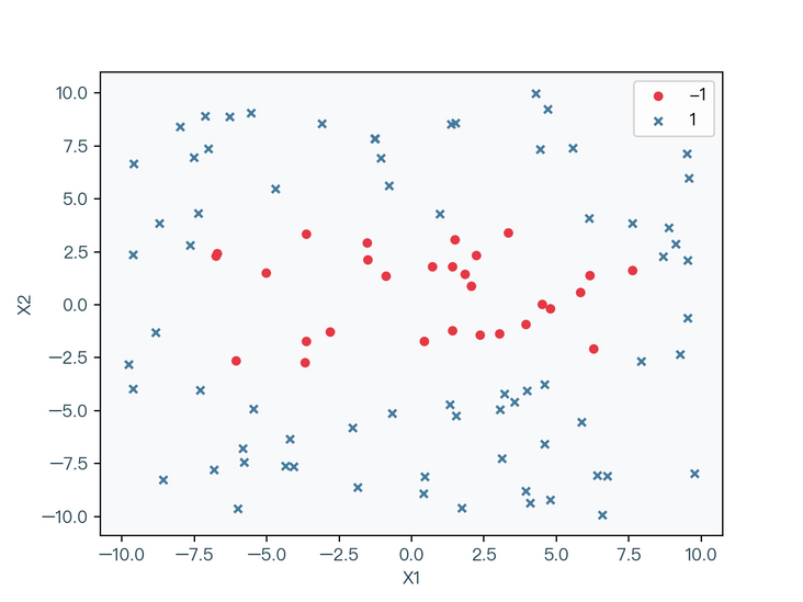
< center > Figure 2-1 < / center >
in Figure 2-1, circles and crosses are used to represent different label classifications respectively. Obviously, the data set cannot be correctly classified by a straight line, but as shown in Figure 2-2, the data set can be correctly classified by an elliptic curve.
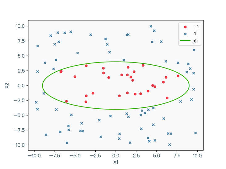
< center > figure 2-2 < / center >
however, it is relatively difficult to solve the problem of nonlinear classification such as elliptic curve in Figure 2-2. Since the linear classification problem is relatively easy to solve, can the data be transformed into a linear classification data through certain nonlinear changes? The answer is yes.
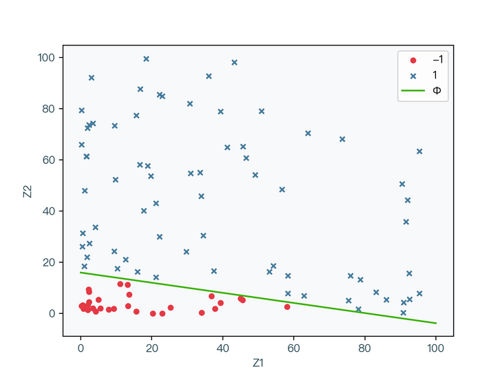
< center > figure 2-3 < / center >
as shown in Fig. 2-3, the data set is subjected to nonlinear transformation (Z = X * X). At this time, it can be seen that the transformed data can be correctly classified through a straight line. The original elliptic curve in Fig. 2-2 is transformed into a straight line in Fig. 2-3, and the original nonlinear classification problem is transformed into a linear classification problem.
Original model
let's review the original model of soft interval support vector machine:
$$ \begin{array}{c} \underset{w, b, \xi}{\min} \frac{1}{2} w^{T} w+C \sum_{i=1}^{N} \xi_{i} \\ \text { s.t. } \quad C>0 \quad \xi_{i} \geq 0 \quad \xi_{i} \geq 1-y_{i}\left(w^{T} x_{i}+b\right) \quad i=1,2, \cdots, N \end{array} $$
< center > formula 2-1 < / center >
suppose there is a φ Function can transform x, for example, mapping x to z in the above example and bringing it into the original model of soft interval support vector machine above:
$$ \begin{array}{c} \underset{w, b, \xi}{\min} \frac{1}{2} w^{T} w+C \sum_{i=1}^{N} \xi_{i} \\ \text { s.t. } \quad C>0 \quad \xi_{i} \geq 0 \quad \xi_{i} \geq 1-y_{i}\left(w^{T} \phi(x_{i})+b\right) \quad i=1,2, \cdots, N \end{array} $$
< center > formula 2-2 < / center >
equation 2-2 above is the original model of nonlinear support vector machine.
Dual model
with the dual model solved in the previous two sections, the dual model of nonlinear support vector machine can be obtained:
$$ \begin{array}{c} \underset{\lambda}{\max} \sum_{i=1}^{N} \lambda_{i}-\frac{1}{2} \sum_{i=1}^{N} \sum_{j=1}^{N} \lambda_{i} \lambda_{j} y_{i} y_{j} \phi(x_{i})^{T} \phi(x_{j}) \\ \text { s.t. } \quad \sum_{i=1}^{N} \lambda_{i} y_{i}=0 \quad 0 \leq \lambda_{i} \leq C \quad i=1,2, \cdots, N \end{array} $$
< center > formula 2-3 < / center >
Nuclear technique
observe the change part of the dual model of soft interval support vector machine in equation 2-3, and the feature vector passes through φ After the function transformation, its dimension may be very high, and it is usually difficult to find the inner product. In order to bypass this inner product calculation, we can find a function as shown in equation 2-4, so that the value calculated by the function is equal to the inner product after feature conversion. Such a function is called Kernel Function, and this replacement method is called Nuclear technique2(Kernel Trick)
$$ K(x_i, x_j) = \phi(x_i)^T\phi(x_j) $$
< center > formula 2-4 < / center >
use the kernel technique to bring in equation 2-3 to obtain the final dual model of nonlinear support vector machine:
$$ \begin{array}{c} \underset{\lambda}{\max} \sum_{i=1}^{N} \lambda_{i}-\frac{1}{2} \sum_{i=1}^{N} \sum_{j=1}^{N} \lambda_{i} \lambda_{j} y_{i} y_{j} K(x_i, x_j) \\ \text { s.t. } \quad \sum_{i=1}^{N} \lambda_{i} y_{i}=0 \quad 0 \leq \lambda_{i} \leq C \quad i=1,2, \cdots, N \end{array} $$
< center > formula 2-5 < / center >
decision making under nuclear technology:
(1) Original decision surface function
(2) Weight coefficient w
(3) The final decision surface function is obtained by using kernel technique
$$ \begin{aligned} f(x) &=w^{T} \phi(x)+b & (1)\\ &=\sum_{i=1}^{N} \lambda_{i} y_{i} \phi\left(x_{i}\right) \phi(x)+b & (2)\\ &=\sum_{i=1}^{N} \lambda_{i} y_{i} K\left(x_{i}, x\right)+b & (3) \end{aligned} $$
< center > formula 2-6 < / center >
kernel technique is not only applicable to support vector machines, but also widely used in other machine learning algorithms.
kernel function
common kernel functions:
(1) Linear Kernel: the classification result of support vector machine using Linear Kernel is the same as that of soft interval support vector machine
(2) Polynomial Kernel: when γ = 1, ε = When 0, d = 1, the Polynomial Kernel function degenerates into a linear kernel function
(3) Radial basis function/RBF Kernel: the common Gaussian Kernel is a kind of radial basis function
(4) Sigmoid Kernel: tanh is a hyperbolic tangent function
$$ \begin{aligned} K\left(x_{i}, x_{j}\right)&=x_{i}^{T} x_{j} & (1) \\ K\left(x_{i}, x_{j}\right)&=\left(\gamma x_{i}^{T} x_{j}+\varepsilon\right)^{d} & (2)\\ K\left(x_{i}, x_{j}\right)&=e^{-\gamma\left\|x_{i}-x_{j}\right\|^{2}} & (3)\\ K\left(x_{i}, x_{j}\right)&=\tanh \left(\gamma x_{i}^{T} x_{j}+\varepsilon\right) & (4) \end{aligned} $$
< center > formula 2-7 < / center >
3, Algorithm steps
compared with the dual model of soft interval support vector machine, nonlinear support vector machine only uses kernel function to replace the inner product of feature vector, and the others have no change, so the corresponding sequence minimum optimization algorithm (SMO) has little change.
for the algorithm steps, please refer to the contents in the previous two sections and the following code implementation. At the same time, you can refer to Corresponding papers of SMO algorithm 3. Implementation.
4, Code implementation
Using Python to implement nonlinear support vector machine (SMO algorithm)
import numpy as np

class SMO:
    """
    Support vector machine
    Implementation of sequential minimum optimization algorithm( Sequential minimal optimization/SMO)
    """

    def __init__(self, X, y, kernel, degree = 3, coef0 = 0.0, gamma = 1.0):
        # Training sample characteristic matrix (N * p)
        self.X = X
        # Training sample label vector (N * 1)
        self.y = y
        # Lagrange multiplier vector (N * 1)
        self.alpha = np.zeros(X.shape[0])
        # Error vector, default to negative label vector (N * 1)
        self.errors = -y
        # Offset
        self.b = 0
        # Generation value
        self.cost = -np.inf
        # kernel function
        self.kernel = kernel
        # Kernel related parameters
        self.degree = degree
        self.coef0 = coef0
        self.gamma = gamma

    def fit(self, C = 1, tol = 1e-4):
        """
        Algorithm from John C. Platt My thesis
        https://www.microsoft.com/en-us/research/uploads/prod/1998/04/sequential-minimal-optimization.pdf
        """
        # Update change times
        numChanged = 0
        # Check all
        examineAll = True
        while numChanged > 0 or examineAll:
            numChanged = 0
            if examineAll:
                for idx in range(X.shape[0]):
                    numChanged += self.update(idx, C)
            else:
                for idx in range(X.shape[0]):
                    if self.alpha[idx] <= 0:
                        continue
                    numChanged += self.update(idx, C)
            if examineAll:
                examineAll = False
            elif numChanged == 0:
                examineAll = True
            # Calculate generation value
            cost = self.calcCost()
            if self.cost > 0:
                # The algorithm ends when the change of contemporary value is less than the allowable range
                rate = (cost - self.cost) / self.cost
                if rate <= tol:
                    break
            self.cost = cost

    def update(self, idx, C = 1):
        """
        Subscript for idx The Lagrange multiplier is updated
        """
        X = self.X
        y = self.y
        alpha = self.alpha
        # Check whether the current Lagrange multiplier meets the KKT condition. If it meets the condition, it will directly return 0
        if self.checkKKT(idx, C):
            return 0
        if len(alpha[(alpha != 0)]) > 1:
            # Find the subscript of the second Lagrange multiplier to be optimized according to the principle of | E1 - E2 | maximum
            jdx = self.selectJdx(idx)
            # Update the Lagrange multipliers with subscripts idx and jdx, and return 1 directly when the update is successful
            if self.updateAlpha(idx, jdx, C):
                return 1
        # When the update is not successful, the Lagrange multiplier that is not zero is traversed for update
        for jdx in range(X.shape[0]):
            if alpha[jdx] == 0:
                continue
            # Update the Lagrange multipliers with subscripts idx and jdx, and return 1 directly when the update is successful
            if self.updateAlpha(idx, jdx, C):
                return 1
        # When the update is still unsuccessful, the Lagrange multiplier traversing zero is updated
        for jdx in range(X.shape[0]):
            if alpha[jdx] != 0:
                continue
            # Update the Lagrange multipliers with subscripts idx and jdx, and return 1 directly when the update is successful
            if self.updateAlpha(idx, jdx, C):
                return 1
        # Return 0 if there is still no update
        return 0

    def selectJdx(self, idx):
        """
        Find the subscript of the second Lagrange multiplier to be optimized
        """
        errors = self.errors
        if errors[idx] > 0:
            # When the error term is greater than zero, select the subscript of the minimum value in the error vector
            return np.argmin(errors)
        elif errors[idx] < 0:
            # When the error term is less than zero, select the subscript of the maximum value in the error vector
            return np.argmax(errors)
        else:
            # When the error term is equal to zero, select the subscript with the largest absolute value of the maximum and minimum value in the error vector
            minJdx = np.argmin(errors)
            maxJdx = np.argmax(errors)
            if max(np.abs(errors[minJdx]), np.abs(errors[maxJdx])) - errors[minJdx]:
                return minJdx
            else:
                return maxJdx

    def calcB(self):
        """
        Calculate offset
        Calculate the offset corresponding to each Lagrange multiplier that is not zero, and then take its average value
        """
        X = self.X
        y = self.y
        alpha = self.alpha
        alpha_gt = alpha[alpha > 0]
        # Non zero quantity in Lagrange multiplier vector
        alpha_gt_len = len(alpha_gt)
        # Returns 0 directly when all are zero
        if alpha_gt_len == 0:
            return 0
        # b = y - Wx, please refer to the description in the article for the specific algorithm
        X_gt = X[alpha > 0]
        y_gt = y[alpha > 0]

        s = 0
        for idx in range(X_gt.shape[0]):
            ss = 0
            for jdx in range(X_gt.shape[0]):
                ss += alpha_gt[jdx] * y_gt[jdx] * self.kernel(X_gt[jdx], X_gt[idx], self.degree, self.coef0, self.gamma)
            s += y_gt[idx] - ss
        return s / alpha_gt_len

    def calcCost(self):
        """
        Calculate generation value
        It can be calculated according to the algorithm in the article
        """
        X = self.X
        y = self.y
        alpha = self.alpha
        cost = 0
        for idx in range(X.shape[0]):
            for jdx in range(X.shape[0]):
                cost = cost + (y[idx] * y[jdx] * self.kernel(X[idx], X[jdx], self.degree, self.coef0, self.gamma) * alpha[idx] * alpha[jdx])
        return np.sum(alpha) - cost / 2

    def checkKKT(self, idx, C = 1):
        """
        Check subscript is idx Is the Lagrange multiplier satisfied KKT condition
        1. alpha >= 0
        2. alpha <= C
        3. y * f(x) - 1 >= 0
        4. alpha * (y * f(x) - 1) = 0
        """
        y = self.y
        errors = self.errors
        alpha = self.alpha
        r = errors[idx] * y[idx]
        if (alpha[idx] > 0 and alpha[idx] < C and r == 0) or (alpha[idx] == 0 and r > 0) or (alpha[idx] == C and r < 0):
            return True
        return False

    def calcU(self, idx, jdx, C = 1):
        """
        Calculate the upper bound of Lagrange multiplier so that the two Lagrange multipliers to be optimized are greater than or equal to 0 at the same time
        It can be calculated according to the algorithm in the article
        """
        y = self.y
        alpha = self.alpha
        if y[idx] * y[jdx] == 1:
            return max(0, alpha[jdx] + alpha[idx] - C)
        else:
            return max(0.0, alpha[jdx] - alpha[idx])

    def calcV(self, idx, jdx, C = 1):
        """
        Calculate the lower bound of Lagrange multiplier so that the two Lagrange multipliers to be optimized are greater than or equal to 0 at the same time
        It can be calculated according to the algorithm in the article
        """
        y = self.y
        alpha = self.alpha
        if y[idx] * y[jdx] == 1:
            return min(C, alpha[jdx] + alpha[idx])
        else:
            return min(C, C + alpha[jdx] - alpha[idx])

    def updateAlpha(self, idx, jdx, C = 1):
        """
        Subscript for idx,jdx The Lagrange multiplier is updated
        It can be calculated according to the algorithm in the article
        """
        if idx == jdx:
            return False
        X = self.X
        y = self.y
        alpha = self.alpha
        errors = self.errors
        # Error term of idx
        Ei = errors[idx]
        # Error term of jdx
        Ej = errors[jdx]
        U = self.calcU(idx, jdx, C)
        V = self.calcV(idx, jdx, C)
        if U == V:
            return False
        Kii = self.kernel(X[idx], X[idx], self.degree, self.coef0, self.gamma)
        Kjj = self.kernel(X[jdx], X[jdx], self.degree, self.coef0, self.gamma)
        Kij = self.kernel(X[idx], X[jdx], self.degree, self.coef0, self.gamma)
        # Calculate K
        K = Kii + Kjj - 2 * Kij
        oldAlphaIdx = alpha[idx]
        oldAlphaJdx = alpha[jdx]
        oldB = self.b
        s = y[idx] * y[jdx]
        if K > 0:
            # Calculating the new Lagrange multiplier of jdx
            newAlphaJdx = oldAlphaJdx + y[jdx] * (Ei - Ej) / K
            if newAlphaJdx < U:
                # When the new value exceeds the upper bound, change it to the upper bound
                newAlphaJdx = U
            if newAlphaJdx > V:
                # When the new value is lower than the lower bound, change it to the lower bound
                newAlphaJdx = V
        else:
            fi = y[idx] * (Ei + oldB) - oldAlphaIdx * Kii - s * oldAlphaJdx * Kij
            fj = y[jdx] * (Ej + oldB) - s * oldAlphaIdx * Kij - oldAlphaJdx * Kjj
            Vv = oldAlphaIdx + s * (oldAlphaJdx - V)
            Uu = oldAlphaIdx + s * (oldAlphaJdx - U)
            Vv = Vv * fi + V * fj + 0.5 * (Vv ** 2) * Kii + 0.5 * (V ** 2) * Kjj + s * V * Vv * Kij
            Uu = Uu * fi + U * fj + 0.5 * (Uu ** 2) * Kii + 0.5 * (U ** 2) * Kjj + s * U * Uu * Kij
            if Vv < Uu:
                newAlphaJdx = V
            elif Vv > Uu:
                newAlphaJdx = U
            else:
                newAlphaJdx = oldAlphaJdx
        if oldAlphaJdx == newAlphaJdx:
            # When the new value is equal to the old value, it is judged as not updated and returned directly
            return False
        # New Lagrange multipliers for computing idx
        newAlphaIdx = oldAlphaIdx + s * (oldAlphaJdx - newAlphaJdx)
        # Update Lagrange multiplier vector
        alpha[idx] = newAlphaIdx
        alpha[jdx] = newAlphaJdx
        oldB = self.b
        # Recalculate offset
        self.b = self.calcB()
        # Recalculate error vector
        newErrors = []
        for i in range(X.shape[0]):
            newError = errors[i] + y[idx] * (newAlphaIdx - oldAlphaIdx) * self.kernel(X[idx], X[i], self.degree, self.coef0, self.gamma) + y[jdx] * (newAlphaJdx - oldAlphaJdx) * self.kernel(X[jdx], X[i]) - oldB + self.b
            newErrors.append(newError)
        self.errors = newErrors
        return True

    def predict(self, X):
        fxs = []
        for idx in range(len(X)):
            fx = 0
            for jdx in range(self.X.shape[0]):
                fx += self.y[jdx] * self.alpha[jdx] * self.kernel(self.X[jdx], X[idx], self.degree, self.coef0, self.gamma)
            fxs.append(fx + self.b)
        return np.sign(fxs)
Linear kernel support vector machine
# Linear kernel support vector machine
def linearKernel(x, z, degree = 3, coef0 = 0.0, gamma = 1.0):
    return x.dot(z)

linearSmo = SMO(X, y, kernel = linearKernel)
linearSmo.fit()
Polynomial kernel support vector machine
# Polynomial kernel support vector machine
def polynomialKernel(x, z, degree = 3, coef0 = 0.0, gamma = 1.0):
    return np.power(gamma * x.dot(z) + coef0, degree)

polynomialSmo = SMO(X, y, kernel = polynomialKernel)
polynomialSmo.fit()
Radial basis function kernel support vector machine
# Radial basis function kernel support vector machine
def rbfKernel(x, z, degree = 3, coef0 = 0.0, gamma = 1.0):
    return np.exp(-gamma * np.power(np.linalg.norm(x - z), 2))

rbfSmo = SMO(X, y, kernel = rbfKernel)
rbfSmo.fit()
5, Third party library implementation
scikit-learn 4 implementation
from sklearn.svm import SVC

# Linear kernel support vector machine
svc = SVC(kernel = "linear")
# Polynomial kernel support vector machine
svc = SVC(kernel = "poly", gamma = 1)
# Radial basis function kernel support vector machine
svc = SVC(kernel = "rbf", gamma = 1)

# Fitting data
svc.fit(X, y)
Scikit learn uses LIBSVM 5 library. For details about the implementation of this library, please refer to This article6 .
6, Animation demonstration
the following three figures respectively show the classification results of linearly indivisible data sets for different kernel functions. Red represents the sample points with label value of - 1 and blue represents the sample points with label value of 1. The light red area is the part with the predicted value of - 1, and the light blue area is the part with the predicted value of 1:

< center > figure 6-1 < / center >

< center > figure 6-2 < / center >
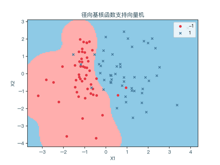
< center > figure 6-3 < / center >
it can be seen that different kernel functions have a great impact on the classification results. When the form of feature transformation is not known, it is impossible to select the appropriate kernel function. However, generally, for nonlinear classification problems, radial basis function kernel function can be used to find the appropriate parameters through cross verification.
7, Mind map

< center > Figure 7-1 < / center >
8, References
- https://en.wikipedia.org/wiki...
- https://en.wikipedia.org/wiki...
- https://www.microsoft.com/en-...
- https://scikit-learn.org/stab...
- https://www.csie.ntu.edu.tw/~...
- https://github.com/Kaslanaria...
For a complete demonstration, please click here
Note: This article strives to be accurate and easy to understand, but as the author is also a beginner, his level is limited. If there are errors or omissions in the article, readers are urged to criticize and correct it by leaving a message
This article was first published in—— AI map , welcome to pay attention