Background knowledge required for reading this article: hard interval support vector machine, relaxation variables, yidui programming knowledge
1, Introduction
in the previous section, we introduced a most basic support vector machine model - hard interval support vector machine. This model can classify linearly separable data sets, but in reality, data sets are often linearly non separable. In this section, we will introduce the second one of support vector machines—— Soft interval support vector machine 1 (soft margin support vector machine) to solve the problem of linear indivisibility of data sets mentioned above.
Two, model introduction
Original model
let's first look at the original model of hard interval support vector machine as follows:
$$ \begin{array}{} \underset{w, b}{\max} \frac{1}{2} w^Tw \\ \text { s.t. } \quad y_{i}\left(w^{T} x_{i}+b\right) \geq 1 \quad i=1,2, \cdots, N \end{array} $$
< center > formula 2-1 < / center >
the constraint y(wx + b) is greater than or equal to 1 to make all sample points under the correct classification, which is why it is called hard interval. At present, the data sets cannot be completely separated by a hyperplane, so it is necessary to allow some data sets not to meet the above constraints.
modify the above cost function and add the penalty term of sample points with wrong classification, in which 1(x) is mentioned in the previous chapter, i.e Indicator function 2 (indicator function). When the following inequality is satisfied, the function returns 1, and when it is not satisfied, the function returns 0. At the same time, the punishment force is controlled by the constant C, where C > 0. It can be seen that when C is infinite, it will force each sample point to be classified correctly, which is equivalent to hard interval support vector machine.
$$ \begin{array}{} \underset{w, b}{\min} \frac{1}{2} w^{T} w+C \sum_{i=1}^{N} 1_{x_{i}}\left(y_{i}\left(w^{T} x_{i}+b\right) \lt 1\right) \\ \text { s.t. } \quad C>0 \end{array} $$
< center > formula 2-2 < / center >
the indicator function in equation 2-2 is neither convex nor continuous, which is troublesome to handle. At this time, it can be replaced by max function, in the form as follows:
$$ \begin{array}{} \underset{w, b}{\min} \frac{1}{2} w^{T} w+C \sum_{i=1}^{N} \max\left(0, 1 - y_{i}\left(w^{T} x_{i}+b\right)\right) \\ \text { s.t. } \quad C>0 \end{array} $$
< center > formula 2-3 < / center >
it will be introduced at this time Relaxation variable 3(slack variable) ξ, At the same time, add the following conditions to further remove the max function. Equation 2-3 is the original model of soft interval support vector machine:
$$ \begin{array}{} \underset{w, b, \xi}{\min} \frac{1}{2} w^{T} w+C \sum_{i=1}^{N} \xi_{i} \\ \text { s.t. } \quad C>0 \quad \xi_{i} \geq 0 \quad \xi_{i} \geq 1-y_{i}\left(w^{T} x_{i}+b\right) \quad i=1,2, \cdots, N \end{array} $$
< center > formula 2-4 < / center >
Dual model
like the processing method of hard interval support vector machine, the original model is transformed by Lagrange multiplier method:
(1) Using Lagrange multiplier method, two kinds of Lagrange parameters are introduced λ,μ, Lagrange function is obtained
(2) The Lagrange function takes the partial derivative of w and makes it zero
(3) The analytical solution of w is obtained as hard interval support vector machine
(4) The Lagrange function takes the partial derivative of b and makes it zero
(5) Lagrange function pair ξ Find the partial derivative and make it zero
(6) Get C= λ + μ
$$ \begin{aligned} L(w, b, \xi, \lambda, \mu) &=\frac{1}{2} w^{T} w+C \sum_{i=1}^{N} \xi_{i}+\sum_{i=1}^{N} \lambda_{i}\left(1-\xi_{i}-y_{i}\left(w^{T} x_{i}+b\right)\right)-\sum_{i=1}^{N} \mu_{i} \xi_{i} & (1)\\ \frac{\partial L}{\partial w} &=w-\sum_{i=1}^{N} \lambda_{i} y_{i} x_{i}=0 & (2)\\ w &=\sum_{i=1}^{N} \lambda_{i} y_{i} x_{i} & (3)\\ \frac{\partial L}{\partial b} &=\sum_{i=1}^{N} \lambda_{i} y_{i}=0 & (4)\\ \frac{\partial L}{\partial \xi_{i}} &=C-\lambda_{i}-\mu_{i}=0 & (5)\\ C &=\lambda_{i}+\mu_{i} & (6) \end{aligned} $$
< center > formula 2-5 < / center >
bring the results obtained from equation 2-5 back to the Lagrange function:
(1) Lagrange function
(2) Bring in and expand parentheses
(3) It can be seen that in formula (2), items 2 and 5 cancel each other, items 3 and 8 cancel each other, and item 7 is zero. After combination, it is obtained
$$ \begin{aligned} L(w, b, \xi, \lambda, \mu) &=\frac{1}{2} w^{T} w+C \sum_{i=1}^{N} \xi_{i}+\sum_{i=1}^{N} \lambda_{i}\left(1-\xi_{i}-y_{i}\left(w^{T} x_{i}+b\right)\right)-\sum_{i=1}^{N} \mu_{i} \xi_{i} & (1)\\ &=\frac{1}{2} \sum_{i=1}^{N} \sum_{j=1}^{N} \lambda_{i} \lambda_{j} y_{i} y_{j} x_{i}^{T} x_{i}+\sum_{i=1}^{N} \lambda_{i} \xi_{i}+\sum_{i=1}^{N} \mu_{i} \xi_{i}+\sum_{i=1}^{N} \lambda_{i}-\sum_{i=1}^{N} \lambda_{i} \xi_{i}-\sum_{i=1}^{N} \sum_{j=1}^{N} \lambda_{i} \lambda_{j} y_{i} y_{j} x_{i}^{T} x_{i}-\sum_{i=1}^{N} \lambda_{i} y_{i} b-\sum_{i=1}^{N} \mu_{i} \xi_{i} & (2)\\ &=\sum_{i=1}^{N} \lambda_{i}-\frac{1}{2} \sum_{i=1}^{N} \sum_{j=1}^{N} \lambda_{i} \lambda_{j} y_{i} y_{j} x_{i}^{T} x_{i} & (3) \end{aligned} $$
< center > formula 2-6 < / center >
let's look at the conditions of Lagrange multiplier parameters:
(1) Lagrange multiplier μ Restrictions on
(2) Add Lagrange Multipliers on both sides at the same time λ
(3) Combined with the result of formula 2-5 (6), the
$$ \begin{aligned} \mu_i &\ge 0 & (1) \\ \lambda_i + \mu_i &\ge \lambda_i & (2) \\ C &\ge \lambda_i & (3) \end{aligned} $$
< center > formula 2-7 < / center >
like hard interval support vector machine, KKT conditions are introduced as follows:
$$ \left\{\begin{aligned} \nabla_{w, b, \xi} L(w, b, \xi, \lambda, \mu) &=0 \\ \lambda_{i} & \geq 0 \\ y_{i}\left(w^{T} x_{i}+b\right)-1+\xi_{i} & \geq 0 \\ \lambda_{i}\left(y_{i}\left(w^{T} x_{i}+b\right)-1+\xi_{i}\right) &=0 \\ \mu_{i} & \geq 0 \\ \xi_{i} & \geq 0 \\ \mu_{i} \xi_{i} &=0 \end{aligned}\right. $$
< center > formula 2-8 < / center >
after using the Lagrange multiplier method, the Lagrange dual model of the original model is obtained, and the KKT conditions shown above need to be met:
$$ \begin{array}{} \underset{\lambda}{\max} \sum_{i=1}^{N} \lambda_{i}-\frac{1}{2} \sum_{i=1}^{N} \sum_{j=1}^{N} \lambda_{i} \lambda_{j} y_{i} y_{j} x_{i}^{T} x_{j} \\ \text { s.t. } \quad \sum_{i=1}^{N} \lambda_{i} y_{i}=0 \quad 0 \leq \lambda_{i} \leq C \quad i=1,2, \cdots, N \end{array} $$
< center > formula 2-9 < / center >
3, Algorithm steps
after comparing the dual model of equation 2-9 above with the dual model of hard interval support vector machine, it will be found that the difference between them lies in the different constraints of Lagrange multiplier. The former only has an upper bound of penalty factor C, so its solution algorithm is roughly the same as that of hard interval support vector machine, except for the following two differences.
one change in the algorithm is the new algorithm λ_ Calculation of upper and lower bounds of b:
(1) (2) all λ Must be greater than or equal to zero and less than or equal to C
(3) Case by case discussion λ_ b. restrictions
(4) The final variable is obtained by synthesizing formula (1) λ_ b. restrictions
$$ \begin{aligned} &0 \leq \lambda_{b}^{\text {new }} \leq C & (1)\\ &0 \leq \lambda_{a}^{\text {old }}+y_{a} y_{b}\left(\lambda_{b}^{\text {old }}-\lambda_{b}^{\text {new }}\right) \leq C & (2)\\ \Rightarrow&\left\{\begin{array}{} \lambda_{a}^{\text {old }}+\lambda_{b}^{\text {old }}-C \leq \lambda_{b}^{\text {new }} \leq \lambda_{a}^{\text {old }}+\lambda_{b}^{\text {old }}, \quad y_{a} y_{b}=+1 \\ \lambda_{b}^{\text {old }}-\lambda_{a}^{\text {old }} \leq \lambda_{b}^{\text {new }} \leq C-\lambda_{a}^{\text {old }}+\lambda_{b}^{\text {old }}, \quad y_{a} y_{b}=-1 \end{array}\right. & (3)\\ \Rightarrow&\left\{\begin{array}{} \max \left(0, \lambda_{a}^{\text {old }}+\lambda_{b}^{\text {old }}-C\right) \leq \lambda_{b}^{\text {new }} \leq \min \left(C, \lambda_{a}^{\text {old }}+\lambda_{b}^{\text {old }}\right), \quad y_{a} y_{b}=+1 \\ \max \left(0, \lambda_{b}^{\text {old }}-\lambda_{a}^{\text {old }}\right) \leq \lambda_{b}^{\text {new }} \leq \min \left(C, C-\lambda_{a}^{\text {old }}+\lambda_{b}^{\text {old }}\right), \quad y_{a} y_{b}=-1 \end{array}\right. & (4) \end{aligned} $$
< center > formula 3-1 < / center >
another change in the algorithm is the judgment of KKT condition:
(1) Consider λ Equal to 0
(2) According to the result of (6) in equation 2-5 μ Equal to C
(3) Because μ Equal to C, according to the KKT condition of equation 2-8 ξ Equal to 0
(4) Will ξ Equal to 0 is brought into KKT condition
$$ \begin{aligned} \lambda &=0 & (1)\\ \mu &=C & (2)\\ \xi &=0 & (3)\\ y_{i}\left(w^{T} x_{i}+b\right)-1 & \geq 0 & (4) \end{aligned} $$
< center > formula 3-2 < / center >
(1) Consider λ Equal to C
(2) According to the result of (6) in equation 2-5 μ Equal to 0
(3) Because λ Not equal to 0, according to the KKT condition of equation 2-8
(4) Because ξ Greater than or equal to 0 can be obtained by combining formula (3)
$$ \begin{aligned} \lambda &=C & (1)\\ \mu &=0 & (2)\\ y_{i}\left(w^{T} x_{i}+b\right)-1 + \xi &=0 & (3)\\ y_{i}\left(w^{T} x_{i}+b\right)-1 & \leq 0 & (4) \end{aligned} $$
< center > formula 3-3 < / center >
(1) Consider λ Between 0 and C
(2) According to the result of (6) in equation 2-5 μ Also between 0 and C
(3) According to the KKT condition of equation 2-8
(4) Because λ It is not equal to 0, which can be obtained according to the KKT condition of equation 2-8 and in combination with equation (3)
$$ \begin{aligned} 0 \lt \lambda &\lt C & (1)\\ 0 \lt \mu &\lt C & (2)\\ \xi &=0 & (3)\\ y_{i}\left(w^{T} x_{i}+b\right)-1 & = 0 & (4) \end{aligned} $$
< center > formula 3-4 < / center >
by combining equations 3-2, 3-3 and 3-4 above, the following new restrictions can be obtained:
$$ \left\{\begin{array}{} y_{i}\left(w^{T} x_{i}+b\right)-1 \geq 0, & \lambda=0 \\ y_{i}\left(w^{T} x_{i}+b\right)-1=0, & 0 \lt \lambda \lt C \\ y_{i}\left(w^{T} x_{i}+b\right)-1 \leq 0, & \lambda=C \end{array}\right. $$
< center > formula 3-5 < / center >
for the algorithm steps, please refer to the third section of hard interval support vector machine and the following code implementation.
4, Code implementation
Implementation using Python
import numpy as np

class SMO:
    """
    Soft interval support vector machine
    Implementation of sequential minimum optimization algorithm( Sequential minimal optimization/SMO)
    """

    def __init__(self, X, y):
        # Training sample characteristic matrix (N * p)
        self.X = X
        # Training sample label vector (N * 1)
        self.y = y
        # Lagrange multiplier vector (N * 1)
        self.alpha = np.zeros(X.shape[0])
        # Error vector, default to negative label vector (N * 1)
        self.errors = -y
        # Offset
        self.b = 0
        # Weight vector (p * 1)
        self.w = np.zeros(X.shape[1])
        # Generation value
        self.cost = -np.inf

    def fit(self, C = 1, tol = 1e-4):
        """
        Algorithm from John C. Platt My thesis
        https://www.microsoft.com/en-us/research/uploads/prod/1998/04/sequential-minimal-optimization.pdf
        """
        # Update change times
        numChanged = 0
        # Check all
        examineAll = True
        while numChanged > 0 or examineAll:
            numChanged = 0
            if examineAll:
                for idx in range(X.shape[0]):
                    numChanged += self.update(idx, C)
            else:
                for idx in range(X.shape[0]):
                    if self.alpha[idx] <= 0:
                        continue
                    numChanged += self.update(idx, C)
            if examineAll:
                examineAll = False
            elif numChanged == 0:
                examineAll = True
            # Calculate generation value
            cost = self.calcCost()
            if self.cost > 0:
                # The algorithm ends when the change of contemporary value is less than the allowable range
                rate = (cost - self.cost) / self.cost
                if rate <= tol:
                    break
            self.cost = cost

    def update(self, idx, C = 1):
        """
        Subscript for idx The Lagrange multiplier is updated
        """
        X = self.X
        y = self.y
        alpha = self.alpha
        # Check whether the current Lagrange multiplier meets the KKT condition. If it meets the condition, it will directly return 0
        if self.checkKKT(idx, C):
            return 0
        if len(alpha[(alpha != 0)]) > 1:
            # Find the subscript of the second Lagrange multiplier to be optimized according to the principle of | E1 - E2 | maximum
            jdx = self.selectJdx(idx)
            # Update the Lagrange multipliers with subscripts idx and jdx, and return 1 directly when the update is successful
            if self.updateAlpha(idx, jdx, C):
                return 1
        # When the update is not successful, the Lagrange multiplier that is not zero is traversed for update
        for jdx in range(X.shape[0]):
            if alpha[jdx] == 0:
                continue
            # Update the Lagrange multipliers with subscripts idx and jdx, and return 1 directly when the update is successful
            if self.updateAlpha(idx, jdx, C):
                return 1
        # When the update is still unsuccessful, the Lagrange multiplier traversing zero is updated
        for jdx in range(X.shape[0]):
            if alpha[jdx] != 0:
                continue
            # Update the Lagrange multipliers with subscripts idx and jdx, and return 1 directly when the update is successful
            if self.updateAlpha(idx, jdx, C):
                return 1
        # Return 0 if there is still no update
        return 0

    def selectJdx(self, idx):
        """
        Find the subscript of the second Lagrange multiplier to be optimized
        """
        errors = self.errors
        if errors[idx] > 0:
            # When the error term is greater than zero, select the subscript of the minimum value in the error vector
            return np.argmin(errors)
        elif errors[idx] < 0:
            # When the error term is less than zero, select the subscript of the maximum value in the error vector
            return np.argmax(errors)
        else:
            # When the error term is equal to zero, select the subscript with the largest absolute value of the maximum and minimum value in the error vector
            minJdx = np.argmin(errors)
            maxJdx = np.argmax(errors)
            if max(np.abs(errors[minJdx]), np.abs(errors[maxJdx])) - errors[minJdx]:
                return minJdx
            else:
                return maxJdx

    def calcB(self):
        """
        Calculate offset
        Calculate the offset corresponding to each Lagrange multiplier that is not zero, and then take its average value
        """
        X = self.X
        y = self.y
        alpha = self.alpha
        alpha_gt = alpha[alpha > 0]
        # Non zero quantity in Lagrange multiplier vector
        alpha_gt_len = len(alpha_gt)
        # Returns 0 directly when all are zero
        if alpha_gt_len == 0:
            return 0
        # b = y - Wx, please refer to the description in the article for the specific algorithm
        X_gt = X[alpha > 0]
        y_gt = y[alpha > 0]
        alpha_gt_y = np.array(np.multiply(alpha_gt, y_gt)).reshape(-1, 1)
        s = np.sum(np.multiply(alpha_gt_y, X_gt), axis=0)
        return np.sum(y_gt - X_gt.dot(s)) / alpha_gt_len

    def calcCost(self):
        """
        Calculate generation value
        It can be calculated according to the algorithm in the article
        """
        X = self.X
        y = self.y
        alpha = self.alpha
        cost = 0
        for idx in range(X.shape[0]):
            for jdx in range(X.shape[0]):
                cost = cost + (y[idx] * y[jdx] * X[idx].dot(X[jdx]) * alpha[idx] * alpha[jdx])
        return np.sum(alpha) - cost / 2

    def checkKKT(self, idx, C = 1):
        """
        Check subscript is idx Is the Lagrange multiplier satisfied KKT condition
        1. alpha >= 0
        2. alpha <= C
        3. y * f(x) - 1 >= 0
        4. alpha * (y * f(x) - 1) = 0
        """
        y = self.y
        errors = self.errors
        alpha = self.alpha
        r = errors[idx] * y[idx]
        if (alpha[idx] > 0 and alpha[idx] < C and r == 0) or (alpha[idx] == 0 and r > 0) or (alpha[idx] == C and r < 0):
            return True
        return False

    def calcE(self):
        """
        Calculate error vector
        E = f(x) - y
        """
        X = self.X
        y = self.y
        alpha = self.alpha
        alpha_y = np.array(np.multiply(alpha, y)).reshape(-1, 1)
        errors = X.dot(X.T).dot(alpha_y).T[0] + self.b - y
        return errors

    def calcU(self, idx, jdx, C = 1):
        """
        Calculate the upper bound of Lagrange multiplier so that the two Lagrange multipliers to be optimized are greater than or equal to 0 at the same time
        It can be calculated according to the algorithm in the article
        """
        y = self.y
        alpha = self.alpha
        if y[idx] * y[jdx] == 1:
            return max(0, alpha[jdx] + alpha[idx] - C)
        else:
            return max(0.0, alpha[jdx] - alpha[idx])

    def calcV(self, idx, jdx, C = 1):
        """
        Calculate the lower bound of Lagrange multiplier so that the two Lagrange multipliers to be optimized are greater than or equal to 0 at the same time
        It can be calculated according to the algorithm in the article
        """
        y = self.y
        alpha = self.alpha
        if y[idx] * y[jdx] == 1:
            return min(C, alpha[jdx] + alpha[idx])
        else:
            return min(C, C + alpha[jdx] - alpha[idx])

    def updateAlpha(self, idx, jdx, C = 1):
        """
        Subscript for idx,jdx The Lagrange multiplier is updated
        It can be calculated according to the algorithm in the article
        """
        if idx == jdx:
            return False
        X = self.X
        y = self.y
        alpha = self.alpha
        errors = self.errors
        # Error term of idx
        Ei = errors[idx]
        # Error term of jdx
        Ej = errors[jdx]
        Kii = X[idx].dot(X[idx])
        Kjj = X[jdx].dot(X[jdx])
        Kij = X[idx].dot(X[jdx])
        # Calculate K
        K = Kii + Kjj - 2 * Kij
        oldAlphaIdx = alpha[idx]
        oldAlphaJdx = alpha[jdx]
        # Calculating the new Lagrange multiplier of jdx
        newAlphaJdx = oldAlphaJdx + y[jdx] * (Ei - Ej) / K
        U = self.calcU(idx, jdx, C)
        V = self.calcV(idx, jdx, C)
        if newAlphaJdx < U:
            # When the new value exceeds the upper bound, change it to the upper bound
            newAlphaJdx = U
        if newAlphaJdx > V:
            # When the new value is lower than the lower bound, change it to the lower bound
            newAlphaJdx = V
        if oldAlphaJdx == newAlphaJdx:
            # When the new value is equal to the old value, it is judged as not updated and returned directly
            return False
        # New Lagrange multipliers for computing idx
        newAlphaIdx = oldAlphaIdx + y[idx] * y[jdx] * (oldAlphaJdx - newAlphaJdx)
        # Update weight vector
        self.w = self.w + y[idx] * (newAlphaIdx - oldAlphaIdx) * X[idx] + y[jdx] * (newAlphaJdx - oldAlphaJdx) * X[jdx]
        # Update Lagrange multiplier vector
        alpha[idx] = newAlphaIdx
        alpha[jdx] = newAlphaJdx
        oldB = self.b
        # Recalculate offset
        self.b = self.calcB()
        # Recalculate error vector
        eps = np.finfo(np.float32).eps
        newErrors = []
        for i in range(X.shape[0]):
            newError = errors[i] + y[idx] * (newAlphaIdx - oldAlphaIdx) * X[idx].dot(X[i]) + y[jdx] * (newAlphaJdx - oldAlphaJdx) * X[jdx].dot(X[i]) - oldB + self.b
            if np.abs(newError) < eps:
                newError = 0
            newErrors.append(newError)
        self.errors = newErrors
        return True
5, Third party library implementation
scikit-learn 4 implementation
from sklearn.svm import SVC

svc = SVC(kernel = "linear", C = 1)
# Fitting data
svc.fit(X, y)
# weight coefficient
w = svc.coef_
# intercept
b = svc.intercept_
print("w", w, "b", b)
6, Animation demonstration
the following figure shows a linearly inseparable data set, in which red represents the sample point with label value of - 1 and blue represents the sample point with label value of 1:
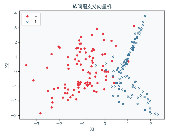
< center > figure 6-1 < / center >
the following figure shows the results of fitting data by soft interval support vector machine. The light red area is the part with the predicted value of - 1, and the light blue area is the part with the predicted value of 1:

< center > figure 6-2 < / center >
7, Mind map
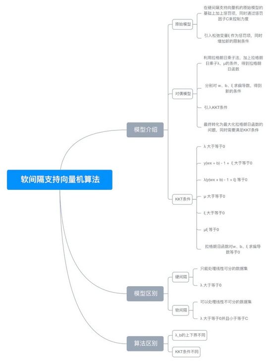
< center > Figure 7-1 < / center >
8, References
- https://en.wikipedia.org/wiki...
- https://en.wikipedia.org/wiki...
- https://en.wikipedia.org/wiki...
- https://scikit-learn.org/stab...
For a complete demonstration, please click here
Note: This article strives to be accurate and easy to understand, but as the author is also a beginner, his level is limited. If there are errors or omissions in the article, readers are urged to criticize and correct it by leaving a message
This article was first published in—— AI map , welcome to pay attention