First, let me make an advertisement~
If you need more artificial intelligence courses (source code + Notes + courseware), please scan the QR code to get it

The following is the text
In order to facilitate the exchange of fans, a Q group was established: [809160367,] let's learn and exchange together, including courseware materials, source code sharing and Daniel's problem solving.
Generally speaking, there are three algorithms for machine learning:
1. Supervised learning
Supervised learning algorithm includes a target variable (i.e. dependent variable) and a predictive variable (equivalent to independent variable) used to predict the target variable Through these variables, we can build a model, so that for an independent variable, we can get the corresponding dependent variable The model is trained repeatedly until it can achieve the desired accuracy on the training data set
Supervised learning algorithms include regression model, decision tree, random forest, K-nearest neighbor algorithm, logical regression and so on
2. Unsupervised algorithm
The difference between unsupervised learning and unsupervised learning is that we have no dependent variables to predict or estimate Unsupervised learning is used to classify the overall object It plays a wide role in classifying customers according to a certain index
The unsupervised learning algorithms include association rules, K-means clustering algorithm and so on
3. Reinforcement learning
This algorithm can train the program to make a decision. The program tries all possible behaviors in a certain situation, records the results of different actions, and tries to find the best attempt to make a decision
Algorithms belonging to reinforcement learning include: Markov decision process
Common machine learning algorithms include:
1. Linear regression
2. Logistic regression
3. Decision tree
4. Support vector machine (SVM)
5. Naive Bayes
6.K-nearest neighbor algorithm (KNN)
7.K-means algorithm
8. Random forest
9. Dimensional reduction algorithms
10.Gradient Boost and Adaboost algorithms
One by one:
1. Linear regression
Linear regression uses continuous variables to estimate actual values (such as house prices). We find the best linear relationship between independent variables and dependent variables through linear regression algorithm, and we can determine the best straight line graphically The best straight line is the regression line The linear regression relationship can be expressed by Y=ax+b
In the formula Y=ax+b:
Y = dependent variable
a = slope
x = independent variable
b = intercept
a and b can be obtained by minimizing the sum of squares of dependent variable errors (least square method)
We can imagine a scenario to understand linear regression For example, you ask a fifth grade child to queue up the students in the class from light to heavy without asking their specific weight. What would the child do? He may line up by observing everyone's height and physique. This is linear regression! The child actually thinks that height and physique are related to people's weight. And this relationship is like the relationship between Y and X in the previous paragraph.
Draw a diagram for you to understand. The linear regression equation used in the figure below is Y=0.28x+13.9 Through this equation, a person's weight information can be predicted according to his height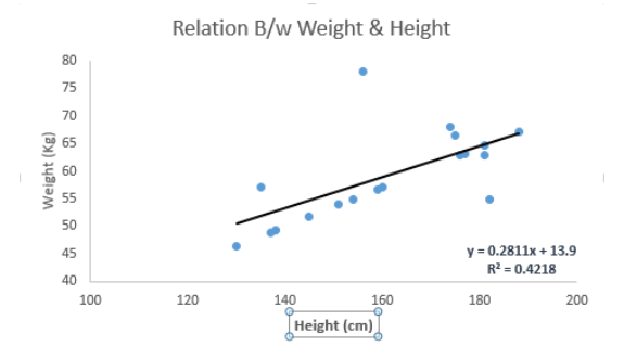
Linear regression is also divided into univariate linear regression and multivariate linear regression Obviously, a single variable has only one independent variable, and a multiple variable has multiple independent variables
When fitting multiple linear regression, polynomial regression or curve regression can be used
Import Library
from sklearn import linear_model

x_train=input_variables_values_training_datasets
y_train=target_variables_values_training_datasets
x_test=input_variables_values_test_datasets

# Create linear regression object
linear = linear_model.LinearRegression()

# Train the model using the training sets and check score
linear.fit(x_train, y_train)
linear.score(x_train, y_train)

#Equation coefficient and Intercept
print('Coefficient: \n', linear.coef_)
print('Intercept: \n', linear.intercept_)

#Predict Output
predicted= linear.predict(x_test)
2. Logistic regression
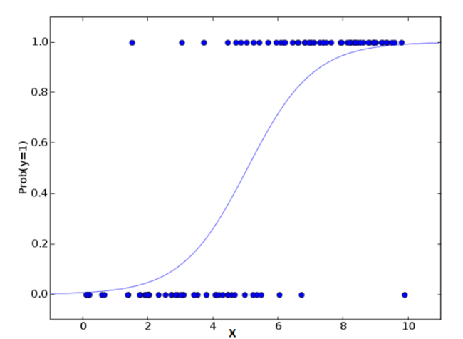
When I first heard about logistic regression, I thought it was a regression algorithm. In fact, it was a classification algorithm. Don't confuse his name Known independent variables are usually used to predict the value of a discrete dependent variable (usually the value of two classifications) In short, he predicts the probability of occurrence at a time by fitting an Lg, so he predicts a probability value, and the value is between 0-1. It is impossible to go out of this range, unless you encounter a false logistic regression!
Also use examples to understand:
Suppose a friend of yours asks you to answer a question. There are only two possible outcomes: you get it right or you don't. In order to study the subject field you are best at, you have done topics in various fields. Then the result of this research may be as follows: if it is a tenth grade trigonometric function problem, you have 70% of the possible performance to solve it. But if it's a fifth grade history problem, the probability that you will is only 30%. Logistic regression gives you such a probability result.
Mathematics is coming again. The industry of algorithm is inseparable from mathematics. You'd better study mathematics well
The linear combination of predictive variables of the final event is:
odds= p/ (1-p) = probability of event occurrence / probability of not event occurrence

ln(odds) = ln(p/(1-p))

logit(p) = ln(p/(1-p)) = b0+b1X1+b2X2+b3X3....+bkXk
Here, p is the probability of the event of interest Instead of minimizing the sum of squares of errors like ordinary regression, he estimates the parameters by screening out specific parameter values to maximize the probability of the observed sample values
As for some people will ask, why do we need to do logarithms? In short, this is the best way to repeat the step function
from sklearn.linear_model import LogisticRegression

 model = LogisticRegression()

 # Train the model using the training sets and check score
 model.fit(X, y)
 model.score(X, y)

 #Equation coefficient and Intercept
 print('Coefficient: \n', model.coef_)
 print('Intercept: \n', model.intercept_)

 #Predict Output
 predicted= model.predict(x_test)
Optimization of logistic regression:
Add interactive item
Reduce characteristic variables
Regularization
Using nonlinear models
3. Decision tree
This is my favorite and frequently used algorithm. It belongs to supervised learning and is often used to solve classification problems. Surprisingly, it can be applied to both categorical variables and continuous variables. This algorithm allows us to divide a population into two or more groups. The grouping is based on the most important characteristic variables / independent variables that can distinguish the population.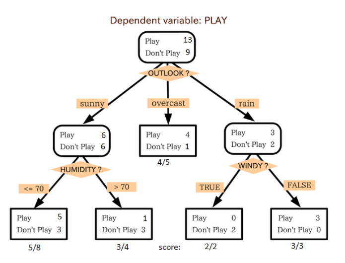
As can be seen from the above figure, the overall crowd is finally divided into four groups in terms of whether to play or not. The grouping is realized according to some characteristic variables. There are many specific indicators for grouping, such as Gini, information gain, chi square and entropy.
from sklearn import tree


# Create tree object
model = tree.DecisionTreeClassifier(criterion='gini') # for classification, here you can change the algorithm as gini or entropy (information gain) by default it is gini

# model = tree.DecisionTreeRegressor() for regression

# Train the model using the training sets and check score
model.fit(X, y)
model.score(X, y)

#Predict Output
predicted= model.predict(x_test)
4. Support vector machine (SVM)
This is a classification algorithm. In this algorithm, we plot each data as a point in an n-dimensional space (n is the characteristic number), and each eigenvalue represents the size of the corresponding coordinate value. For example, we have two characteristics: a person's height and hair length. We can plot these two variables in a two-dimensional space, and each point on the graph has two coordinate values (these axes are also called support vectors).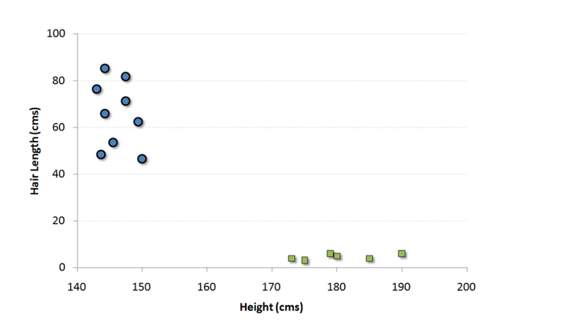
Now we need to find a line in the graph that can separate different groups of points to the greatest extent. In both sets of data, the distance from the nearest point to the line should be the farthest.
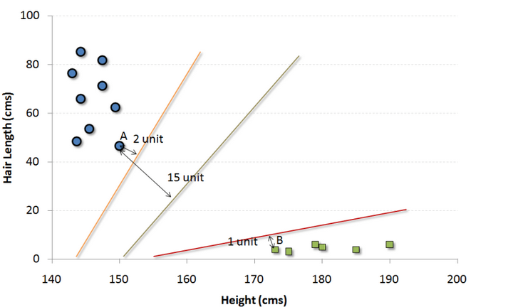
In the above figure, the black line is the best division line. Because this line is farthest from the nearest point in both groups, points A and B are the farthest. Any other line must bring one of the points closer than this distance. In this way, we can classify the data according to which side of the line the data points are distributed.
#Import Library
from sklearn import svm
#Assumed you have, X (predictor) and Y (target) for training data set and x_test(predictor) of test_dataset
# Create SVM classification object

model = svm.svc() # there is various option associated with it, this is simple for classification. You can refer link, for mo# re detail.

# Train the model using the training sets and check score
model.fit(X, y)
model.score(X, y)

#Predict Output
predicted= model.predict(x_test)
5. Naive Bayes
This algorithm is a classification method based on Bayesian theory. Its assumption is that the independent variables are independent of each other. In short, naive Bayes assumes that the occurrence of one feature is independent of other features. For example, if a fruit is red, round and about 7cm in diameter, we may guess it is an apple. Even if there is a certain relationship between these features, in the naive Bayesian algorithm, we all believe that red, round and diameter are independent of each other in judging the possibility that a fruit is an apple.
Naive Bayesian model is easy to build and efficient in analyzing a large number of data problems. Although the model is simple, it works better than very complex classification methods in many cases.
Bayesian theory tells us how to calculate a posteriori probability P(c|x) from a priori probability P(c),P(x) and conditional probability P(x|c). The algorithm is as follows: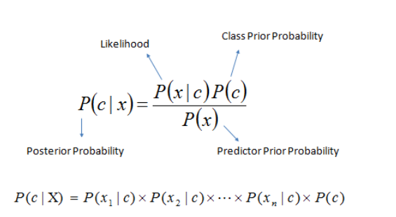
P(c|x) is a posteriori probability classified as C with known feature X.
P(c) is a priori probability of type C.
P(x|c) is the possibility that species C has characteristic X.
P(x) is the a priori probability of characteristic X.
Example: the following training set includes the weather variable and the target variable "whether to go out". We now need to divide people into two groups according to the weather: play or not. The whole process is carried out according to the following steps:
Step 1: make a frequency table according to the known data
Step 2: calculate the probability of each situation and make a probability table. For example, the probability of Overcast is 0.29, and the probability of playing is 0.64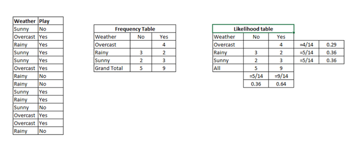
Step 3: use naive Bayes to calculate the a posteriori probability of playing and not playing in each weather condition. The result with high probability is the predicted value.
Question: when the weather is sunny, people will play. Is this statement correct?
We can answer this question in the above way. P(Yes | Sunny)=P(Sunny | Yes) * P(Yes) / P(Sunny).
Here, P(Sunny |Yes) = 3/9 = 0.33, P(Sunny) = 5/14 = 0.36, P(Yes)= 9/14 = 0.64.
Then, P (yes | sunny) = 0.33 * 0.64 / 0.36 = 0.60 > 0.5, indicating that this probability value is greater.
#Import Library
from sklearn.naive_bayes import GaussianNB
#Assumed you have, X (predictor) and Y (target) for training data set and x_test(predictor) of test_dataset

# Create SVM classification object model = GaussianNB() # there is other distribution for multinomial classes like Bernoulli Naive Bayes, Refer link

# Train the model using the training sets and check score
model.fit(X, y)

#Predict Output
predicted= model.predict(x_test)
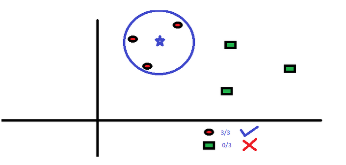
6.KNN (K-proximity algorithm)
This algorithm can solve both classification problems and regression problems, but it is more used in industry. KNN first records all known data, then uses a distance function to find the K group of data closest to the unknown event in the known data, and finally predicts the event according to the most common category in the K group of data.
The distance function can be Euclidean distance, Manhattan distance, Minkowski distance, and Hamming Distance. The first three are used for continuous variables, and Hamming Distance is used to classify variables. If K=1, the problem is simplified to classify according to the latest data. The selection of K value is often the key in KNN modeling.
KNN is widely used in life. For example, if you want to know someone you don't know, you may learn about him from his good friends and circles.
Before using KNN, you need to consider:
The calculation cost of KNN is very high
All features should be normalized by orders of magnitude, otherwise features with large orders of magnitude will be offset in the calculated distance.
Preprocess data before KNN, such as removing outliers, noise, etc.
#Import Library
from sklearn.neighbors import KNeighborsClassifier

#Assumed you have, X (predictor) and Y (target) for training data set and x_test(predictor) of test_dataset
# Create KNeighbors classifier object model

KNeighborsClassifier(n_neighbors=6) # default value for n_neighbors is 5

# Train the model using the training sets and check score
model.fit(X, y)

#Predict Output
predicted= model.predict(x_test)
7. K-Means algorithm
This is an unsupervised learning algorithm to solve the clustering problem. This method simply uses a certain number of clusters (assuming K clusters) to classify the given data. The data points in the same cluster are the same, and the data points in different clusters are different.
Remember how you recognized shapes from ink stains? The process of K-means algorithm is similar. You should also judge the number of clusters by observing the shape and distribution of clusters!

How the K-means algorithm divides clusters:
-
Select K data points from each cluster as centroids.
-
Divide each data point and its nearest centroid into the same cluster, that is, generate K new clusters.
-
Find out the centroid of the new cluster, so there is a new centroid.
-
Repeat 2 and 3 until the results converge, that is, no new centroids appear.
-
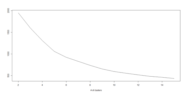
How to determine the value of K:
If we calculate the sum of squares of distances from all points in the cluster to the centroid in each cluster, and then add the sum of squares of distances of different clusters, we will get the total sum of squares of the cluster scheme.
We know that as the number of clusters increases, the total sum of squares decreases. However, if you plot K with the total sum of squares, you will find that the total sum of squares decreases rapidly before a certain value of K, but the reduction range after this value of K decreases greatly. This value is the optimal number of clusters.
#Import Library
from sklearn.cluster import KMeans

#Assumed you have, X (attributes) for training data set and x_test(attributes) of test_dataset
# Create KNeighbors classifier object model
k_means = KMeans(n_clusters=3, random_state=0)

# Train the model using the training sets and check score
model.fit(X)

#Predict Output
predicted= model.predict(x_test)
8. Random forest
Random forest is a unique name for a set of decision trees. In the random forest, we have multiple decision trees (so called "forest"). In order to classify a new observation, each decision tree will give a classification according to its characteristics. The random forest algorithm selects the classification with the most votes as the classification result.How to generate a decision tree:
If there are N categories in the training set, N samples are randomly selected repeatedly. These samples will form a training set to cultivate the decision tree.
If there are m characteristic variables, select the number m < < m, so as to randomly select m characteristic variables on each node to segment the node. M remains constant throughout the forest.
Each decision tree is segmented to the greatest extent without pruning.
#Import Library
from sklearn.ensemble import RandomForestClassifier
#Assumed you have, X (predictor) and Y (target) for training data set and x_test(predictor) of test_dataset

# Create Random Forest object
model= RandomForestClassifier()

# Train the model using the training sets and check score
model.fit(X, y)

#Predict Output
predicted= model.predict(x_test)
9. Dimensional reduction algorithms
In the past 4-5 years, the available data has increased almost exponentially. Companies / government agencies / research organizations not only have more data sources, but also obtain more dimensional data information.For example, e-commerce companies have more detailed information about customers, such as personal information, Internet browsing history, personal likes and dislikes, purchase records, feedback information, etc. they pay attention to your personal characteristics and know you better than the clerk in the supermarket you go to every day.
As a data scientist, the data we have has many characteristics. Although this sounds conducive to building more powerful and accurate models, they are sometimes a big problem in modeling. How can we find the most important variable from 1000 or 2000 variables? In this case, the descending dimension algorithm and other algorithms, such as decision tree, random forest, PCA, factor analysis, correlation matrix, and default value ratio, can help us solve the problem.
#Import Library
from sklearn import decomposition
#Assumed you have training and test data set as train and test
# Create PCA obeject pca= decomposition.PCA(n_components=k) #default value of k =min(n_sample, n_features)
# For Factor analysis
#fa= decomposition.FactorAnalysis()
# Reduced the dimension of training dataset using PCA

train_reduced = pca.fit_transform(train)

#Reduced the dimension of test dataset
test_reduced = pca.transform(test)
10. Gradient boosting and AdaBoost
Both GBM and AdaBoost are boosting algorithms to improve the prediction accuracy when there is a large amount of data. Boosting is an integrated learning method. It improves the prediction accuracy by orderly combining the estimation results of multiple weak classifiers / estimators. These boosting algorithms have played an outstanding role in data science competitions such as Kaggle, AV hackthon and crowdanalytix.
#Import Library
from sklearn.ensemble import GradientBoostingClassifier
#Assumed you have, X (predictor) and Y (target) for training data set and x_test(predictor) of test_dataset
# Create Gradient Boosting Classifier object
model= GradientBoostingClassifier(n_estimators=100, learning_rate=1.0, max_depth=1, random_state=0)

# Train the model using the training sets and check score
model.fit(X, y)
#Predict Output
predicted= model.predict(x_test)