Case 1 (happiness prediction)
Background introduction
Happiness involves philosophy, psychology, sociology, economics and other disciplines. At the same time, it is closely related to everyone's life. Everyone has his own measurement standard for happiness. If we can find the commonalities that affect happiness and find the policy factors that affect happiness, we can optimize the allocation of resources to improve people's happiness. At present, social science research focuses on the interpretability of variables and the implementation of future policies, mainly using the methods of linear regression and logical regression, in terms of economic and demographic factors such as income, health, occupation, social relations and leisure style; And government public services, macroeconomic environment, tax burden and other macro factors.
Specifically, we need to use 139 dimensions of information including individual variables (gender, age, region, occupation, health, marriage and political outlook, etc.), family variables (parents, spouses, children, family capital, etc.), social attitudes (fairness, credit, public services, etc.) to predict their impact on well-being.
Data source: official China Comprehensive Social Survey (CGSS)
Data information
The case requires the use of 139 dimensional features and more than 8000 groups of data to predict personal well-being (the predicted values are 1, 2, 3, 4 and 5, of which 1 represents the lowest well-being and 5 represents the highest well-being).
Considering the large number of variables and the complex relationship between some variables, the data are divided into full version and simplified version. You can start with the simplified version, get familiar with the competition questions, and use the full version to mine more information. The full version of the data is used directly here. The question also gives the questionnaire title corresponding to each variable in the index file and the meaning of variable value; The survey document is the original questionnaire as a supplement to facilitate the understanding of the question background.
evaluating indicator
The final evaluation index is the mean square error MSE, namely:
S
c
o
r
e
=
1
n
∑
1
n
(
y
i
−
y
∗
)
2
Score = \frac{1}{n} \sum_1 ^n (y_i - y ^*)^2
Score=n11∑n(yi−y∗)2
Guide Package
Aside: there are many guide bags here, and the operation is as fierce as a tiger. Please wait patiently, "ah, this damn sweet burden"
import os
import time
import pandas as pd
import numpy as np
import seaborn as sns
from sklearn.linear_model import LogisticRegression
from sklearn.svm import SVC, LinearSVC
from sklearn.ensemble import RandomForestClassifier
from sklearn.neighbors import KNeighborsClassifier
from sklearn.naive_bayes import GaussianNB
from sklearn.linear_model import Perceptron
from sklearn.linear_model import SGDClassifier
from sklearn.tree import DecisionTreeClassifier
from sklearn import metrics
from datetime import datetime
import matplotlib.pyplot as plt
from sklearn.metrics import roc_auc_score, roc_curve, mean_squared_error,mean_absolute_error, f1_score
import lightgbm as lgb
import xgboost as xgb
from sklearn.ensemble import RandomForestRegressor as rfr
from sklearn.ensemble import ExtraTreesRegressor as etr
from sklearn.linear_model import BayesianRidge as br
from sklearn.ensemble import GradientBoostingRegressor as gbr
from sklearn.linear_model import Ridge
from sklearn.linear_model import Lasso
from sklearn.linear_model import LinearRegression as lr
from sklearn.linear_model import ElasticNet as en
from sklearn.kernel_ridge import KernelRidge as kr
from sklearn.model_selection import  KFold, StratifiedKFold,GroupKFold, RepeatedKFold
from sklearn.model_selection import train_test_split
from sklearn.model_selection import GridSearchCV
from sklearn import preprocessing
import logging
import warnings

warnings.filterwarnings('ignore') #Eliminate warning
Import dataset
train = pd.read_csv("train.csv", parse_dates=['survey_time'],encoding='latin-1')
test = pd.read_csv("test.csv", parse_dates=['survey_time'],encoding='latin-1') #latin-1 downward compatible with ASCII
train = train[train["happiness"]!=-8].reset_index(drop=True) #Delete the line whose "happiness" is - 8
train_data_copy = train.copy() # copy
target_col = "happiness" #Target column
target = train_data_copy[target_col]
del train_data_copy[target_col] #Remove target column

data = pd.concat([train_data_copy,test],axis=0,ignore_index=True)
View basic information of data
train.happiness.describe() #Basic information of data
count    7988.000000
mean        3.867927
std         0.818717
min         1.000000
25%         4.000000
50%         4.000000
75%         4.000000
max         5.000000
Name: happiness, dtype: float64
Data preprocessing
Process the continuous negative values in the data. Since the negative values in the data are only - 1, - 2, - 3 and - 8, they operate separately. The implementation code is as follows:
#make feature +5
#There are negative values in csv: - 1, - 2, - 3, - 8, which are regarded as problematic features, but they are not deleted
def getres1(row):
    return len([x for x in row.values if type(x)==int and x<0])

def getres2(row):
    return len([x for x in row.values if type(x)==int and x==-8])

def getres3(row):
    return len([x for x in row.values if type(x)==int and x==-1])

def getres4(row):
    return len([x for x in row.values if type(x)==int and x==-2])

def getres5(row):
    return len([x for x in row.values if type(x)==int and x==-3])

#Check data
data['neg1'] = data[data.columns].apply(lambda row:getres1(row),axis=1)
data.loc[data['neg1']>20,'neg1'] = 20  #Smoothing, up to 20 occurrences

data['neg2'] = data[data.columns].apply(lambda row:getres2(row),axis=1)
data['neg3'] = data[data.columns].apply(lambda row:getres3(row),axis=1)
data['neg4'] = data[data.columns].apply(lambda row:getres4(row),axis=1)
data['neg5'] = data[data.columns].apply(lambda row:getres5(row),axis=1)
Fill in the missing value, fill in the missing value, and use fillna(value), where the value is determined according to the specific situation.
For example, consider most of the missing information as zero, the number of family members as 1, and the characteristic of family income as 66365, that is, the average income of all families. Some implementation codes are as follows:
#Fill in 25 columns of missing values. Remove 4 columns and fill in 21 columns
#The following columns are all default and filled as appropriate
data['work_status'] = data['work_status'].fillna(0)
data['work_yr'] = data['work_yr'].fillna(0)
data['work_manage'] = data['work_manage'].fillna(0)
data['work_type'] = data['work_type'].fillna(0)

data['edu_yr'] = data['edu_yr'].fillna(0)
data['edu_status'] = data['edu_status'].fillna(0)

data['s_work_type'] = data['s_work_type'].fillna(0)
data['s_work_status'] = data['s_work_status'].fillna(0)
data['s_political'] = data['s_political'].fillna(0)
data['s_hukou'] = data['s_hukou'].fillna(0)
data['s_income'] = data['s_income'].fillna(0)
data['s_birth'] = data['s_birth'].fillna(0)
data['s_edu'] = data['s_edu'].fillna(0)
data['s_work_exper'] = data['s_work_exper'].fillna(0)

data['minor_child'] = data['minor_child'].fillna(0)
data['marital_now'] = data['marital_now'].fillna(0)
data['marital_1st'] = data['marital_1st'].fillna(0)
data['social_neighbor']=data['social_neighbor'].fillna(0)
data['social_friend']=data['social_friend'].fillna(0)
data['hukou_loc']=data['hukou_loc'].fillna(1) #At least 1 indicates registered permanent residence
data['family_income']=data['family_income'].fillna(66365) #Average value after deleting the problem value
Time processing – in two parts:
Firstly, the "continuous" ages are stratified, that is, the ages are divided into six intervals.
Secondly, calculate the specific age. In the Excel table, only the date of birth and the survey time and other information are available. Based on this, calculate the real age of each investigator. The specific implementation code is as follows:
#144+1 =145
#Continue with special column data processing
#Reading happiness_index.xlsx
data['survey_time'] = pd.to_datetime(data['survey_time'], format='%Y-%m-%d',errors='coerce')#Prevent error reporting with different time formats errors='coerce‘
data['survey_time'] = data['survey_time'].dt.year #It's just year. It's convenient to calculate the age
data['age'] = data['survey_time']-data['birth']
# print(data['age'],data['survey_time'],data['birth'])
#Age stratification 145 + 1 = 146
bins = [0,17,26,34,50,63,100]
data['age_bin'] = pd.cut(data['age'], bins, labels=[0,1,2,3,4,5])
Here, because the family income is a continuous value, the mode method cannot be used for processing, and the mean value is directly used to complete the missing value.
The third method is to use the real situation in our daily life. For example, if the characteristic of "religious information" is negative, it is considered as "not believing in religion", and it is considered that the "frequency of participating in religious activities" is 1, that is, it has not participated in religious activities and is supplemented subjectively, which is the most used way in this step.
#Dealing with "religion"
data.loc[data['religion']<0,'religion'] = 1 #1 for not believing in religion
data.loc[data['religion_freq']<0,'religion_freq'] = 1 #1. I've never participated
#Treatment of "education level"
data.loc[data['edu']<0,'edu'] = 4 #junior high school
data.loc[data['edu_status']<0,'edu_status'] = 0
data.loc[data['edu_yr']<0,'edu_yr'] = 0
#Treatment of 'personal income'
data.loc[data['income']<0,'income'] = 0 #Consider no income
#Dealing with "political outlook"
data.loc[data['political']<0,'political'] = 1 #Think it's the masses
#Weight treatment
data.loc[(data['weight_jin']<=80)&(data['height_cm']>=160),'weight_jin']= data['weight_jin']*2
data.loc[data['weight_jin']<=60,'weight_jin']= data['weight_jin']*2  #Personal idea, hahaha, there is no adult of 60 kg
#Height treatment
data.loc[data['height_cm']<150,'height_cm'] = 150 #Actual situation of adults
#Treatment of 'health'
data.loc[data['health']<0,'health'] = 4 #Think it's healthier
data.loc[data['health_problem']<0,'health_problem'] = 4
#Dealing with 'depression'
data.loc[data['depression']<0,'depression'] = 4 #Most people are very few
#Handling of 'media'
data.loc[data['media_1']<0,'media_1'] = 1 #Never
data.loc[data['media_2']<0,'media_2'] = 1
data.loc[data['media_3']<0,'media_3'] = 1
data.loc[data['media_4']<0,'media_4'] = 1
data.loc[data['media_5']<0,'media_5'] = 1
data.loc[data['media_6']<0,'media_6'] = 1
#Processing of 'idle activities'
data.loc[data['leisure_1']<0,'leisure_1'] = 1 #All according to their own ideas
data.loc[data['leisure_2']<0,'leisure_2'] = 5
data.loc[data['leisure_3']<0,'leisure_3'] = 3
Mode is used (mode() is used in the code to correct the abnormal value). Since the feature here is idle activity, it is reasonable to use mode to deal with the missing value. The specific code reference is as follows:
data.loc[data['leisure_4']<0,'leisure_4'] = data['leisure_4'].mode() #Take mode
data.loc[data['leisure_5']<0,'leisure_5'] = data['leisure_5'].mode()
data.loc[data['leisure_6']<0,'leisure_6'] = data['leisure_6'].mode()
data.loc[data['leisure_7']<0,'leisure_7'] = data['leisure_7'].mode()
data.loc[data['leisure_8']<0,'leisure_8'] = data['leisure_8'].mode()
data.loc[data['leisure_9']<0,'leisure_9'] = data['leisure_9'].mode()
data.loc[data['leisure_10']<0,'leisure_10'] = data['leisure_10'].mode()
data.loc[data['leisure_11']<0,'leisure_11'] = data['leisure_11'].mode()
data.loc[data['leisure_12']<0,'leisure_12'] = data['leisure_12'].mode()
data.loc[data['socialize']<0,'socialize'] = 2 #very seldom
data.loc[data['relax']<0,'relax'] = 4 #often
data.loc[data['learn']<0,'learn'] = 1 #Never, ha ha ha
#Deal with 'social'
data.loc[data['social_neighbor']<0,'social_neighbor'] = 0
data.loc[data['social_friend']<0,'social_friend'] = 0
data.loc[data['socia_outing']<0,'socia_outing'] = 1
data.loc[data['neighbor_familiarity']<0,'social_neighbor']= 4
#Treatment of "social equity"
data.loc[data['equity']<0,'equity'] = 4
#Treatment of 'social class'
data.loc[data['class_10_before']<0,'class_10_before'] = 3
data.loc[data['class']<0,'class'] = 5
data.loc[data['class_10_after']<0,'class_10_after'] = 5
data.loc[data['class_14']<0,'class_14'] = 2
#Handling of 'working conditions'
data.loc[data['work_status']<0,'work_status'] = 0
data.loc[data['work_yr']<0,'work_yr'] = 0
data.loc[data['work_manage']<0,'work_manage'] = 0
data.loc[data['work_type']<0,'work_type'] = 0
#Treatment of "social security"
data.loc[data['insur_1']<0,'insur_1'] = 1
data.loc[data['insur_2']<0,'insur_2'] = 1
data.loc[data['insur_3']<0,'insur_3'] = 1
data.loc[data['insur_4']<0,'insur_4'] = 1
data.loc[data['insur_1']==0,'insur_1'] = 0
data.loc[data['insur_2']==0,'insur_2'] = 0
data.loc[data['insur_3']==0,'insur_3'] = 0
data.loc[data['insur_4']==0,'insur_4'] = 0
Take the mean value to complete the missing value (the code is implemented as means()). Here, because the family income is a continuous value, the mode method can no longer be used for processing. Here, the mean value is directly used to complete the missing value. The specific code reference is as follows:
#Treatment of family situation
family_income_mean = data['family_income'].mean()
data.loc[data['family_income']<0,'family_income'] = family_income_mean
data.loc[data['family_m']<0,'family_m'] = 2
data.loc[data['family_status']<0,'family_status'] = 3
data.loc[data['house']<0,'house'] = 1
data.loc[data['car']<0,'car'] = 0
data.loc[data['car']==2,'car'] = 0
data.loc[data['son']<0,'son'] = 1
data.loc[data['daughter']<0,'daughter'] = 0
data.loc[data['minor_child']<0,'minor_child'] = 0
#'marriage 'treatment
data.loc[data['marital_1st']<0,'marital_1st'] = 0
data.loc[data['marital_now']<0,'marital_now'] = 0
#Treatment of 'spouse'
data.loc[data['s_birth']<0,'s_birth'] = 0
data.loc[data['s_edu']<0,'s_edu'] = 0
data.loc[data['s_political']<0,'s_political'] = 0
data.loc[data['s_hukou']<0,'s_hukou'] = 0
data.loc[data['s_income']<0,'s_income'] = 0
data.loc[data['s_work_type']<0,'s_work_type'] = 0
data.loc[data['s_work_status']<0,'s_work_status'] = 0
data.loc[data['s_work_exper']<0,'s_work_exper'] = 0
#Handling of "parents' situation"
data.loc[data['f_birth']<0,'f_birth'] = 1945
data.loc[data['f_edu']<0,'f_edu'] = 1
data.loc[data['f_political']<0,'f_political'] = 1
data.loc[data['f_work_14']<0,'f_work_14'] = 2
data.loc[data['m_birth']<0,'m_birth'] = 1940
data.loc[data['m_edu']<0,'m_edu'] = 1
data.loc[data['m_political']<0,'m_political'] = 1
data.loc[data['m_work_14']<0,'m_work_14'] = 2
#Socioeconomic status compared to peers
data.loc[data['status_peer']<0,'status_peer'] = 2
#Compared with 3 years ago
data.loc[data['status_3_before']<0,'status_3_before'] = 2
#Treatment of 'views'
data.loc[data['view']<0,'view'] = 4
#Treatment of expected annual income
data.loc[data['inc_ability']<=0,'inc_ability']= 2
inc_exp_mean = data['inc_exp'].mean()
data.loc[data['inc_exp']<=0,'inc_exp']= inc_exp_mean #Take the mean value

#Partial feature processing, mode
for i in range(1,9+1):
    data.loc[data['public_service_'+str(i)]<0,'public_service_'+str(i)] = data['public_service_'+str(i)].dropna().mode().values
for i in range(1,13+1):
    data.loc[data['trust_'+str(i)]<0,'trust_'+str(i)] = data['trust_'+str(i)].dropna().mode().values
Data augmentation
In this step, we need to further analyze the relationship between each feature, so as to expand the data. After thinking, the following features are added here: the age of first marriage, the age of recent marriage, whether to remarry, the age of spouse, the age difference of spouse, various income ratios (the income ratio with spouse, the ratio of expected income after ten years to current income, etc.), the ratio of income to living area (including the expected income after ten years, etc.) Social class (social class after 10 years, social class after 14 years, etc.), leisure index, satisfaction index, trust index, etc.
In addition, the normalization of the same province, city and county is also considered.
For example, the average value of income in the same province and city is equal to the individual's indicators relative to others in the same province, city and county. At the same time, it also considers the comparison between peers, that is, the income and health of peers. The specific implementation code is as follows:
#Age of first marriage 147
data['marital_1stbir'] = data['marital_1st'] - data['birth']
#Recent marriage age 148
data['marital_nowtbir'] = data['marital_now'] - data['birth']
#Remarriage 149
data['mar'] = data['marital_nowtbir'] - data['marital_1stbir']
#Spouse age 150
data['marital_sbir'] = data['marital_now']-data['s_birth']
#Age difference between spouses 151
data['age_'] = data['marital_nowtbir'] - data['marital_sbir']

#Income ratio 151 + 7 = 158
data['income/s_income'] = data['income']/(data['s_income']+1)
data['income+s_income'] = data['income']+(data['s_income']+1)
data['income/family_income'] = data['income']/(data['family_income']+1)
data['all_income/family_income'] = (data['income']+data['s_income'])/(data['family_income']+1)
data['income/inc_exp'] = data['income']/(data['inc_exp']+1)
data['family_income/m'] = data['family_income']/(data['family_m']+0.01)
data['income/m'] = data['income']/(data['family_m']+0.01)

#Income / area ratio 158 + 4 = 162
data['income/floor_area'] = data['income']/(data['floor_area']+0.01)
data['all_income/floor_area'] = (data['income']+data['s_income'])/(data['floor_area']+0.01)
data['family_income/floor_area'] = data['family_income']/(data['floor_area']+0.01)
data['floor_area/m'] = data['floor_area']/(data['family_m']+0.01)

#class 162+3=165
data['class_10_diff'] = (data['class_10_after'] - data['class'])
data['class_diff'] = data['class'] - data['class_10_before']
data['class_14_diff'] = data['class'] - data['class_14']

#Leisure index 166
leisure_fea_lis = ['leisure_'+str(i) for i in range(1,13)]
data['leisure_sum'] = data[leisure_fea_lis].sum(axis=1) #skew

#Satisfaction index 167
public_service_fea_lis = ['public_service_'+str(i) for i in range(1,10)]
data['public_service_sum'] = data[public_service_fea_lis].sum(axis=1) #skew

#Trust index 168
trust_fea_lis = ['trust_'+str(i) for i in range(1,14)]
data['trust_sum'] = data[trust_fea_lis].sum(axis=1) #skew

#province mean 168+13=181
data['province_income_mean'] = data.groupby(['province'])['income'].transform('mean').values
data['province_family_income_mean'] = data.groupby(['province'])['family_income'].transform('mean').values
data['province_equity_mean'] = data.groupby(['province'])['equity'].transform('mean').values
data['province_depression_mean'] = data.groupby(['province'])['depression'].transform('mean').values
data['province_floor_area_mean'] = data.groupby(['province'])['floor_area'].transform('mean').values
data['province_health_mean'] = data.groupby(['province'])['health'].transform('mean').values
data['province_class_10_diff_mean'] = data.groupby(['province'])['class_10_diff'].transform('mean').values
data['province_class_mean'] = data.groupby(['province'])['class'].transform('mean').values
data['province_health_problem_mean'] = data.groupby(['province'])['health_problem'].transform('mean').values
data['province_family_status_mean'] = data.groupby(['province'])['family_status'].transform('mean').values
data['province_leisure_sum_mean'] = data.groupby(['province'])['leisure_sum'].transform('mean').values
data['province_public_service_sum_mean'] = data.groupby(['province'])['public_service_sum'].transform('mean').values
data['province_trust_sum_mean'] = data.groupby(['province'])['trust_sum'].transform('mean').values

#city   mean 181+13=194
data['city_income_mean'] = data.groupby(['city'])['income'].transform('mean').values
data['city_family_income_mean'] = data.groupby(['city'])['family_income'].transform('mean').values
data['city_equity_mean'] = data.groupby(['city'])['equity'].transform('mean').values
data['city_depression_mean'] = data.groupby(['city'])['depression'].transform('mean').values
data['city_floor_area_mean'] = data.groupby(['city'])['floor_area'].transform('mean').values
data['city_health_mean'] = data.groupby(['city'])['health'].transform('mean').values
data['city_class_10_diff_mean'] = data.groupby(['city'])['class_10_diff'].transform('mean').values
data['city_class_mean'] = data.groupby(['city'])['class'].transform('mean').values
data['city_health_problem_mean'] = data.groupby(['city'])['health_problem'].transform('mean').values
data['city_family_status_mean'] = data.groupby(['city'])['family_status'].transform('mean').values
data['city_leisure_sum_mean'] = data.groupby(['city'])['leisure_sum'].transform('mean').values
data['city_public_service_sum_mean'] = data.groupby(['city'])['public_service_sum'].transform('mean').values
data['city_trust_sum_mean'] = data.groupby(['city'])['trust_sum'].transform('mean').values

#county  mean 194 + 13 = 207
data['county_income_mean'] = data.groupby(['county'])['income'].transform('mean').values
data['county_family_income_mean'] = data.groupby(['county'])['family_income'].transform('mean').values
data['county_equity_mean'] = data.groupby(['county'])['equity'].transform('mean').values
data['county_depression_mean'] = data.groupby(['county'])['depression'].transform('mean').values
data['county_floor_area_mean'] = data.groupby(['county'])['floor_area'].transform('mean').values
data['county_health_mean'] = data.groupby(['county'])['health'].transform('mean').values
data['county_class_10_diff_mean'] = data.groupby(['county'])['class_10_diff'].transform('mean').values
data['county_class_mean'] = data.groupby(['county'])['class'].transform('mean').values
data['county_health_problem_mean'] = data.groupby(['county'])['health_problem'].transform('mean').values
data['county_family_status_mean'] = data.groupby(['county'])['family_status'].transform('mean').values
data['county_leisure_sum_mean'] = data.groupby(['county'])['leisure_sum'].transform('mean').values
data['county_public_service_sum_mean'] = data.groupby(['county'])['public_service_sum'].transform('mean').values
data['county_trust_sum_mean'] = data.groupby(['county'])['trust_sum'].transform('mean').values

#ratio compared with the same province 207 + 13 = 220
data['income/province'] = data['income']/(data['province_income_mean'])
data['family_income/province'] = data['family_income']/(data['province_family_income_mean'])
data['equity/province'] = data['equity']/(data['province_equity_mean'])
data['depression/province'] = data['depression']/(data['province_depression_mean'])
data['floor_area/province'] = data['floor_area']/(data['province_floor_area_mean'])
data['health/province'] = data['health']/(data['province_health_mean'])
data['class_10_diff/province'] = data['class_10_diff']/(data['province_class_10_diff_mean'])
data['class/province'] = data['class']/(data['province_class_mean'])
data['health_problem/province'] = data['health_problem']/(data['province_health_problem_mean'])
data['family_status/province'] = data['family_status']/(data['province_family_status_mean'])
data['leisure_sum/province'] = data['leisure_sum']/(data['province_leisure_sum_mean'])
data['public_service_sum/province'] = data['public_service_sum']/(data['province_public_service_sum_mean'])
data['trust_sum/province'] = data['trust_sum']/(data['province_trust_sum_mean']+1)

#ratio compared with the same city 220 + 13 = 233
data['income/city'] = data['income']/(data['city_income_mean'])
data['family_income/city'] = data['family_income']/(data['city_family_income_mean'])
data['equity/city'] = data['equity']/(data['city_equity_mean'])
data['depression/city'] = data['depression']/(data['city_depression_mean'])
data['floor_area/city'] = data['floor_area']/(data['city_floor_area_mean'])
data['health/city'] = data['health']/(data['city_health_mean'])
data['class_10_diff/city'] = data['class_10_diff']/(data['city_class_10_diff_mean'])
data['class/city'] = data['class']/(data['city_class_mean'])
data['health_problem/city'] = data['health_problem']/(data['city_health_problem_mean'])
data['family_status/city'] = data['family_status']/(data['city_family_status_mean'])
data['leisure_sum/city'] = data['leisure_sum']/(data['city_leisure_sum_mean'])
data['public_service_sum/city'] = data['public_service_sum']/(data['city_public_service_sum_mean'])
data['trust_sum/city'] = data['trust_sum']/(data['city_trust_sum_mean'])

#ratio compared with 233 + 13 = 246 in the same region
data['income/county'] = data['income']/(data['county_income_mean'])
data['family_income/county'] = data['family_income']/(data['county_family_income_mean'])
data['equity/county'] = data['equity']/(data['county_equity_mean'])
data['depression/county'] = data['depression']/(data['county_depression_mean'])
data['floor_area/county'] = data['floor_area']/(data['county_floor_area_mean'])
data['health/county'] = data['health']/(data['county_health_mean'])
data['class_10_diff/county'] = data['class_10_diff']/(data['county_class_10_diff_mean'])
data['class/county'] = data['class']/(data['county_class_mean'])
data['health_problem/county'] = data['health_problem']/(data['county_health_problem_mean'])
data['family_status/county'] = data['family_status']/(data['county_family_status_mean'])
data['leisure_sum/county'] = data['leisure_sum']/(data['county_leisure_sum_mean'])
data['public_service_sum/county'] = data['public_service_sum']/(data['county_public_service_sum_mean'])
data['trust_sum/county'] = data['trust_sum']/(data['county_trust_sum_mean'])

#age   mean 246+ 13 =259
data['age_income_mean'] = data.groupby(['age'])['income'].transform('mean').values
data['age_family_income_mean'] = data.groupby(['age'])['family_income'].transform('mean').values
data['age_equity_mean'] = data.groupby(['age'])['equity'].transform('mean').values
data['age_depression_mean'] = data.groupby(['age'])['depression'].transform('mean').values
data['age_floor_area_mean'] = data.groupby(['age'])['floor_area'].transform('mean').values
data['age_health_mean'] = data.groupby(['age'])['health'].transform('mean').values
data['age_class_10_diff_mean'] = data.groupby(['age'])['class_10_diff'].transform('mean').values
data['age_class_mean'] = data.groupby(['age'])['class'].transform('mean').values
data['age_health_problem_mean'] = data.groupby(['age'])['health_problem'].transform('mean').values
data['age_family_status_mean'] = data.groupby(['age'])['family_status'].transform('mean').values
data['age_leisure_sum_mean'] = data.groupby(['age'])['leisure_sum'].transform('mean').values
data['age_public_service_sum_mean'] = data.groupby(['age'])['public_service_sum'].transform('mean').values
data['age_trust_sum_mean'] = data.groupby(['age'])['trust_sum'].transform('mean').values

# 259 + 13 = 272 compared to peers
data['income/age'] = data['income']/(data['age_income_mean'])
data['family_income/age'] = data['family_income']/(data['age_family_income_mean'])
data['equity/age'] = data['equity']/(data['age_equity_mean'])
data['depression/age'] = data['depression']/(data['age_depression_mean'])
data['floor_area/age'] = data['floor_area']/(data['age_floor_area_mean'])
data['health/age'] = data['health']/(data['age_health_mean'])
data['class_10_diff/age'] = data['class_10_diff']/(data['age_class_10_diff_mean'])
data['class/age'] = data['class']/(data['age_class_mean'])
data['health_problem/age'] = data['health_problem']/(data['age_health_problem_mean'])
data['family_status/age'] = data['family_status']/(data['age_family_status_mean'])
data['leisure_sum/age'] = data['leisure_sum']/(data['age_leisure_sum_mean'])
data['public_service_sum/age'] = data['public_service_sum']/(data['age_public_service_sum_mean'])
data['trust_sum/age'] = data['trust_sum']/(data['age_trust_sum_mean'])
After the above operations, our features are finally expanded from 131 dimensions to 272 dimensions. Next, we consider the work of Feature Engineering, training model and model fusion.
print('shape',data.shape)
data.head()
shape (10956, 272)
| id | survey_type | province | city | county | survey_time | gender | birth | nationality | religion | ... | depression/age | floor_area/age | health/age | class_10_diff/age | class/age | health_problem/age | family_status/age | leisure_sum/age | public_service_sum/age | trust_sum/age | |
|---|---|---|---|---|---|---|---|---|---|---|---|---|---|---|---|---|---|---|---|---|---|
| 0 | 1 | 1 | 12 | 32 | 59 | 2015 | 1 | 1959 | 1 | 1 | ... | 1.285211 | 0.410351 | 0.848837 | 0.000000 | 0.683307 | 0.521429 | 0.733668 | 0.724620 | 0.666638 | 0.925941 |
| 1 | 2 | 2 | 18 | 52 | 85 | 2015 | 1 | 1992 | 1 | 1 | ... | 0.733333 | 0.952824 | 1.179337 | 1.012552 | 1.344444 | 0.891344 | 1.359551 | 1.011792 | 1.130778 | 1.188442 |
| 2 | 3 | 2 | 29 | 83 | 126 | 2015 | 2 | 1967 | 1 | 0 | ... | 1.343537 | 0.972328 | 1.150485 | 1.190955 | 1.195762 | 1.055679 | 1.190955 | 0.966470 | 1.193204 | 0.803693 |
| 3 | 4 | 2 | 10 | 28 | 51 | 2015 | 2 | 1943 | 1 | 1 | ... | 1.111663 | 0.642329 | 1.276353 | 4.977778 | 1.199143 | 1.188329 | 1.162630 | 0.899346 | 1.153810 | 1.300950 |
| 4 | 5 | 1 | 7 | 18 | 36 | 2015 | 2 | 1994 | 1 | 1 | ... | 0.750000 | 0.587284 | 1.177106 | 0.000000 | 0.236957 | 1.116803 | 1.093645 | 1.045313 | 0.728161 | 1.117428 |
5 rows × 272 columns
We should also delete features with a small number of effective samples, such as features with too many negative values or features with too many missing values. Here, I deleted a total of 9 types of features, including "current highest education level", and got the final 263 dimensional features
#272-9=263
#Delete features with very few values and previously used features
del_list=['id','survey_time','edu_other','invest_other','property_other','join_party','province','city','county']
use_feature = [clo for clo in data.columns if clo not in del_list]
data.fillna(0,inplace=True) #Or make up 0
train_shape = train.shape[0] #Total data volume, training set
features = data[use_feature].columns #All features after deletion
X_train_263 = data[:train_shape][use_feature].values
y_train = target
X_test_263 = data[train_shape:][use_feature].values
X_train_263.shape #The final 263 features
(7988, 263)
Here, the most important 49 features are selected as another group of features in addition to the above 263 Witt signs
imp_fea_49 = ['equity','depression','health','class','family_status','health_problem','class_10_after',
           'equity/province','equity/city','equity/county',
           'depression/province','depression/city','depression/county',
           'health/province','health/city','health/county',
           'class/province','class/city','class/county',
           'family_status/province','family_status/city','family_status/county',
           'family_income/province','family_income/city','family_income/county',
           'floor_area/province','floor_area/city','floor_area/county',
           'leisure_sum/province','leisure_sum/city','leisure_sum/county',
           'public_service_sum/province','public_service_sum/city','public_service_sum/county',
           'trust_sum/province','trust_sum/city','trust_sum/county',
           'income/m','public_service_sum','class_diff','status_3_before','age_income_mean','age_floor_area_mean',
           'weight_jin','height_cm',
           'health/age','depression/age','equity/age','leisure_sum/age'
          ]
train_shape = train.shape[0]
X_train_49 = data[:train_shape][imp_fea_49].values
X_test_49 = data[train_shape:][imp_fea_49].values
X_train_49.shape #The 49 most important features
(7988, 49)
Select the discrete variables that need onehot coding for one hot coding, and then combine them into the third type of features, a total of 383 dimensions.
cat_fea = ['survey_type','gender','nationality','edu_status','political','hukou','hukou_loc','work_exper','work_status','work_type',
           'work_manage','marital','s_political','s_hukou','s_work_exper','s_work_status','s_work_type','f_political','f_work_14',
           'm_political','m_work_14']
noc_fea = [clo for clo in use_feature if clo not in cat_fea]

onehot_data = data[cat_fea].values
enc = preprocessing.OneHotEncoder(categories = 'auto')
oh_data=enc.fit_transform(onehot_data).toarray()
oh_data.shape #Change to onehot encoding format

X_train_oh = oh_data[:train_shape,:]
X_test_oh = oh_data[train_shape:,:]
X_train_oh.shape #Training set

X_train_383 = np.column_stack([data[:train_shape][noc_fea].values,X_train_oh])#First noc, then cat_fea
X_test_383 = np.column_stack([data[train_shape:][noc_fea].values,X_test_oh])
X_train_383.shape
(7988, 383)
Based on this, we have constructed and completed three feature projects (training data sets). One is the most important 49 features extracted above, including health, social class, income among peers and so on. The second is the expanded 263 dimensional feature (which can be considered as the initial feature here). The third is the feature after using one hot coding. The reason for using one hot coding here is that some features are separated values, such as men and women in gender, men are 1 and women are 2. We want to use one hot to change it into men are 0 and women are 1 to enhance the robustness of machine learning algorithm; Another example is the feature of nationality, which originally had 56 values of 1-56. If it is classified directly, the robustness of the classifier will become worse, so it is changed into six features by using one hot coding for non-zero or one processing.
Feature modeling
Firstly, we use lightGBM to process the original 263 dimensional features. Here, we use the method of 5-fold cross verification:
1.lightGBM
##### lgb_263 #
#GBM decision tree
lgb_263_param = {
'num_leaves': 7,
'min_data_in_leaf': 20, #The minimum number of records a leaf may have
'objective':'regression',
'max_depth': -1,
'learning_rate': 0.003,
"boosting": "gbdt", #Using gbdt algorithm
"feature_fraction": 0.18, #For example, 0.18 means that 18% of the parameters are randomly selected in each iteration to build the tree
"bagging_freq": 1,
"bagging_fraction": 0.55, #Data scale used in each iteration
"bagging_seed": 14,
"metric": 'mse',
"lambda_l1": 0.1005,
"lambda_l2": 0.1996,
"verbosity": -1}
folds = StratifiedKFold(n_splits=5, shuffle=True, random_state=4)   #Cross segmentation: 5
oof_lgb_263 = np.zeros(len(X_train_263))
predictions_lgb_263 = np.zeros(len(X_test_263))

for fold_, (trn_idx, val_idx) in enumerate(folds.split(X_train_263, y_train)):

    print("fold n°{}".format(fold_+1))
    trn_data = lgb.Dataset(X_train_263[trn_idx], y_train[trn_idx])
    val_data = lgb.Dataset(X_train_263[val_idx], y_train[val_idx])#train:val=4:1

    num_round = 10000
    lgb_263 = lgb.train(lgb_263_param, trn_data, num_round, valid_sets = [trn_data, val_data], verbose_eval=500, early_stopping_rounds = 800)
    oof_lgb_263[val_idx] = lgb_263.predict(X_train_263[val_idx], num_iteration=lgb_263.best_iteration)
    predictions_lgb_263 += lgb_263.predict(X_test_263, num_iteration=lgb_263.best_iteration) / folds.n_splits

print("CV score: {:<8.8f}".format(mean_squared_error(oof_lgb_263, target)))
fold n°1
Training until validation scores don't improve for 800 rounds
[500]	training's l2: 0.507058	valid_1's l2: 0.50963
[1000]	training's l2: 0.458952	valid_1's l2: 0.469564
[1500]	training's l2: 0.433197	valid_1's l2: 0.453234
[2000]	training's l2: 0.415242	valid_1's l2: 0.444839
[2500]	training's l2: 0.400993	valid_1's l2: 0.440086
[3000]	training's l2: 0.388937	valid_1's l2: 0.436924
[3500]	training's l2: 0.378101	valid_1's l2: 0.434974
[4000]	training's l2: 0.368159	valid_1's l2: 0.43406
[4500]	training's l2: 0.358827	valid_1's l2: 0.433151
[5000]	training's l2: 0.350291	valid_1's l2: 0.432544
[5500]	training's l2: 0.342368	valid_1's l2: 0.431821
[6000]	training's l2: 0.334675	valid_1's l2: 0.431331
[6500]	training's l2: 0.327275	valid_1's l2: 0.431014
[7000]	training's l2: 0.320398	valid_1's l2: 0.431087
[7500]	training's l2: 0.31352	valid_1's l2: 0.430819
[8000]	training's l2: 0.307021	valid_1's l2: 0.430848
[8500]	training's l2: 0.300811	valid_1's l2: 0.430688
[9000]	training's l2: 0.294787	valid_1's l2: 0.430441
[9500]	training's l2: 0.288993	valid_1's l2: 0.430433
Early stopping, best iteration is:
[9119]	training's l2: 0.293371	valid_1's l2: 0.430308
fold n°2
Training until validation scores don't improve for 800 rounds
[500]	training's l2: 0.49895	valid_1's l2: 0.52945
[1000]	training's l2: 0.450107	valid_1's l2: 0.496478
[1500]	training's l2: 0.424394	valid_1's l2: 0.483286
[2000]	training's l2: 0.40666	valid_1's l2: 0.476764
[2500]	training's l2: 0.392432	valid_1's l2: 0.472668
[3000]	training's l2: 0.380438	valid_1's l2: 0.470481
[3500]	training's l2: 0.369872	valid_1's l2: 0.468919
[4000]	training's l2: 0.36014	valid_1's l2: 0.467318
[4500]	training's l2: 0.351175	valid_1's l2: 0.466438
[5000]	training's l2: 0.342705	valid_1's l2: 0.466284
[5500]	training's l2: 0.334778	valid_1's l2: 0.466151
[6000]	training's l2: 0.3273	valid_1's l2: 0.466016
[6500]	training's l2: 0.320121	valid_1's l2: 0.466013
Early stopping, best iteration is:
[5915]	training's l2: 0.328534	valid_1's l2: 0.465918
fold n°3
Training until validation scores don't improve for 800 rounds
[500]	training's l2: 0.499658	valid_1's l2: 0.528985
[1000]	training's l2: 0.450356	valid_1's l2: 0.497264
[1500]	training's l2: 0.424109	valid_1's l2: 0.485403
[2000]	training's l2: 0.405965	valid_1's l2: 0.479513
[2500]	training's l2: 0.391747	valid_1's l2: 0.47646
[3000]	training's l2: 0.379601	valid_1's l2: 0.474691
[3500]	training's l2: 0.368915	valid_1's l2: 0.473648
[4000]	training's l2: 0.359218	valid_1's l2: 0.47316
[4500]	training's l2: 0.350338	valid_1's l2: 0.473043
[5000]	training's l2: 0.341842	valid_1's l2: 0.472719
[5500]	training's l2: 0.333851	valid_1's l2: 0.472779
Early stopping, best iteration is:
[4942]	training's l2: 0.342828	valid_1's l2: 0.472642
fold n°4
Training until validation scores don't improve for 800 rounds
[500]	training's l2: 0.505224	valid_1's l2: 0.508238
[1000]	training's l2: 0.456198	valid_1's l2: 0.473992
[1500]	training's l2: 0.430167	valid_1's l2: 0.461419
[2000]	training's l2: 0.412084	valid_1's l2: 0.454843
[2500]	training's l2: 0.397714	valid_1's l2: 0.450999
[3000]	training's l2: 0.385456	valid_1's l2: 0.448697
[3500]	training's l2: 0.374527	valid_1's l2: 0.446993
[4000]	training's l2: 0.364711	valid_1's l2: 0.44597
[4500]	training's l2: 0.355626	valid_1's l2: 0.445132
[5000]	training's l2: 0.347108	valid_1's l2: 0.44466
[5500]	training's l2: 0.339146	valid_1's l2: 0.444226
[6000]	training's l2: 0.331478	valid_1's l2: 0.443992
[6500]	training's l2: 0.324231	valid_1's l2: 0.444014
Early stopping, best iteration is:
[5874]	training's l2: 0.333372	valid_1's l2: 0.443868
fold n°5
Training until validation scores don't improve for 800 rounds
[500]	training's l2: 0.504304	valid_1's l2: 0.515256
[1000]	training's l2: 0.456062	valid_1's l2: 0.478544
[1500]	training's l2: 0.430298	valid_1's l2: 0.463847
[2000]	training's l2: 0.412591	valid_1's l2: 0.456182
[2500]	training's l2: 0.398635	valid_1's l2: 0.451783
[3000]	training's l2: 0.386609	valid_1's l2: 0.449154
[3500]	training's l2: 0.375948	valid_1's l2: 0.447265
[4000]	training's l2: 0.366291	valid_1's l2: 0.445796
[4500]	training's l2: 0.357236	valid_1's l2: 0.445098
[5000]	training's l2: 0.348637	valid_1's l2: 0.444364
[5500]	training's l2: 0.340736	valid_1's l2: 0.443998
[6000]	training's l2: 0.333154	valid_1's l2: 0.443622
[6500]	training's l2: 0.325783	valid_1's l2: 0.443226
[7000]	training's l2: 0.318802	valid_1's l2: 0.442986
[7500]	training's l2: 0.312164	valid_1's l2: 0.442928
[8000]	training's l2: 0.305691	valid_1's l2: 0.442696
[8500]	training's l2: 0.29935	valid_1's l2: 0.442521
[9000]	training's l2: 0.293242	valid_1's l2: 0.442655
Early stopping, best iteration is:
[8594]	training's l2: 0.298201	valid_1's l2: 0.44238
CV score: 0.45102656
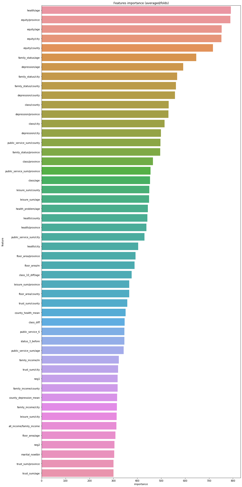
Then, I use the trained lightGBM model to judge and visualize the importance of features. From the results, we can see that health/age ranks first in importance, that is, the health level of peers, which is basically consistent with our subjective views.
#---------------Characteristic importance
pd.set_option('display.max_columns', None)
#Show all rows
pd.set_option('display.max_rows', None)
#Set the display length of value to 100, and the default is 50
pd.set_option('max_colwidth',100)
df = pd.DataFrame(data[use_feature].columns.tolist(), columns=['feature'])
df['importance']=list(lgb_263.feature_importance())
df = df.sort_values(by='importance',ascending=False)
plt.figure(figsize=(14,28))
sns.barplot(x="importance", y="feature", data=df.head(50))
plt.title('Features importance (averaged/folds)')
plt.tight_layout()
Later, we use common machine learning methods to model 263 dimensional features:
2.xgboost
##### xgb_263
#xgboost
xgb_263_params = {'eta': 0.02,  #lr
              'max_depth': 6,
              'min_child_weight':3,#Minimum leaf node sample weight sum
              'gamma':0, #Specifies the minimum loss function drop value required for node splitting.
              'subsample': 0.7,  #Controls the proportion of random samples for each tree
              'colsample_bytree': 0.3,  #It is used to control the proportion of the number of columns sampled randomly per tree (each column is a feature).
              'lambda':2,
              'objective': 'reg:linear',
              'eval_metric': 'rmse',
              'silent': True,
              'nthread': -1}


folds = KFold(n_splits=5, shuffle=True, random_state=2019)
oof_xgb_263 = np.zeros(len(X_train_263))
predictions_xgb_263 = np.zeros(len(X_test_263))

for fold_, (trn_idx, val_idx) in enumerate(folds.split(X_train_263, y_train)):
    print("fold n°{}".format(fold_+1))
    trn_data = xgb.DMatrix(X_train_263[trn_idx], y_train[trn_idx])
    val_data = xgb.DMatrix(X_train_263[val_idx], y_train[val_idx])

    watchlist = [(trn_data, 'train'), (val_data, 'valid_data')]
    xgb_263 = xgb.train(dtrain=trn_data, num_boost_round=3000, evals=watchlist, early_stopping_rounds=600, verbose_eval=500, params=xgb_263_params)
    oof_xgb_263[val_idx] = xgb_263.predict(xgb.DMatrix(X_train_263[val_idx]), ntree_limit=xgb_263.best_ntree_limit)
    predictions_xgb_263 += xgb_263.predict(xgb.DMatrix(X_test_263), ntree_limit=xgb_263.best_ntree_limit) / folds.n_splits

print("CV score: {:<8.8f}".format(mean_squared_error(oof_xgb_263, target)))
fold n°1
[19:14:55] WARNING: /Users/travis/build/dmlc/xgboost/src/objective/regression_obj.cu:170: reg:linear is now deprecated in favor of reg:squarederror.
[19:14:55] WARNING: /Users/travis/build/dmlc/xgboost/src/learner.cc:480:
Parameters: { silent } might not be used.

  This may not be accurate due to some parameters are only used in language bindings but
  passed down to XGBoost core.  Or some parameters are not used but slip through this
  verification. Please open an issue if you find above cases.


[0]	train-rmse:3.40426	valid_data-rmse:3.38329
Multiple eval metrics have been passed: 'valid_data-rmse' will be used for early stopping.

Will train until valid_data-rmse hasn't improved in 600 rounds.
[500]	train-rmse:0.40805	valid_data-rmse:0.70588
[1000]	train-rmse:0.27046	valid_data-rmse:0.70760
Stopping. Best iteration:
[663]	train-rmse:0.35644	valid_data-rmse:0.70521

[19:15:46] WARNING: /Users/travis/build/dmlc/xgboost/src/objective/regression_obj.cu:170: reg:linear is now deprecated in favor of reg:squarederror.
fold n°2
[19:15:46] WARNING: /Users/travis/build/dmlc/xgboost/src/objective/regression_obj.cu:170: reg:linear is now deprecated in favor of reg:squarederror.
[19:15:46] WARNING: /Users/travis/build/dmlc/xgboost/src/learner.cc:480:
Parameters: { silent } might not be used.

  This may not be accurate due to some parameters are only used in language bindings but
  passed down to XGBoost core.  Or some parameters are not used but slip through this
  verification. Please open an issue if you find above cases.


[0]	train-rmse:3.39811	valid_data-rmse:3.40788
Multiple eval metrics have been passed: 'valid_data-rmse' will be used for early stopping.

Will train until valid_data-rmse hasn't improved in 600 rounds.
[500]	train-rmse:0.40719	valid_data-rmse:0.69456
[1000]	train-rmse:0.27402	valid_data-rmse:0.69501
Stopping. Best iteration:
[551]	train-rmse:0.39079	valid_data-rmse:0.69403

[19:16:31] WARNING: /Users/travis/build/dmlc/xgboost/src/objective/regression_obj.cu:170: reg:linear is now deprecated in favor of reg:squarederror.
fold n°3
[19:16:31] WARNING: /Users/travis/build/dmlc/xgboost/src/objective/regression_obj.cu:170: reg:linear is now deprecated in favor of reg:squarederror.
[19:16:31] WARNING: /Users/travis/build/dmlc/xgboost/src/learner.cc:480:
Parameters: { silent } might not be used.

  This may not be accurate due to some parameters are only used in language bindings but
  passed down to XGBoost core.  Or some parameters are not used but slip through this
  verification. Please open an issue if you find above cases.


[0]	train-rmse:3.40181	valid_data-rmse:3.39295
Multiple eval metrics have been passed: 'valid_data-rmse' will be used for early stopping.

Will train until valid_data-rmse hasn't improved in 600 rounds.
[500]	train-rmse:0.41334	valid_data-rmse:0.66250
Stopping. Best iteration:
[333]	train-rmse:0.47284	valid_data-rmse:0.66178

[19:17:07] WARNING: /Users/travis/build/dmlc/xgboost/src/objective/regression_obj.cu:170: reg:linear is now deprecated in favor of reg:squarederror.
fold n°4
[19:17:08] WARNING: /Users/travis/build/dmlc/xgboost/src/objective/regression_obj.cu:170: reg:linear is now deprecated in favor of reg:squarederror.
[19:17:08] WARNING: /Users/travis/build/dmlc/xgboost/src/learner.cc:480:
Parameters: { silent } might not be used.

  This may not be accurate due to some parameters are only used in language bindings but
  passed down to XGBoost core.  Or some parameters are not used but slip through this
  verification. Please open an issue if you find above cases.


[0]	train-rmse:3.40240	valid_data-rmse:3.39012
Multiple eval metrics have been passed: 'valid_data-rmse' will be used for early stopping.

Will train until valid_data-rmse hasn't improved in 600 rounds.
[500]	train-rmse:0.41021	valid_data-rmse:0.66575
[1000]	train-rmse:0.27491	valid_data-rmse:0.66431
Stopping. Best iteration:
[863]	train-rmse:0.30689	valid_data-rmse:0.66358

[19:18:06] WARNING: /Users/travis/build/dmlc/xgboost/src/objective/regression_obj.cu:170: reg:linear is now deprecated in favor of reg:squarederror.
fold n°5
[19:18:07] WARNING: /Users/travis/build/dmlc/xgboost/src/objective/regression_obj.cu:170: reg:linear is now deprecated in favor of reg:squarederror.
[19:18:07] WARNING: /Users/travis/build/dmlc/xgboost/src/learner.cc:480:
Parameters: { silent } might not be used.

  This may not be accurate due to some parameters are only used in language bindings but
  passed down to XGBoost core.  Or some parameters are not used but slip through this
  verification. Please open an issue if you find above cases.


[0]	train-rmse:3.39347	valid_data-rmse:3.42628
Multiple eval metrics have been passed: 'valid_data-rmse' will be used for early stopping.

Will train until valid_data-rmse hasn't improved in 600 rounds.
[500]	train-rmse:0.41704	valid_data-rmse:0.64937
[1000]	train-rmse:0.27907	valid_data-rmse:0.64914
Stopping. Best iteration:
[598]	train-rmse:0.38625	valid_data-rmse:0.64856

[19:18:55] WARNING: /Users/travis/build/dmlc/xgboost/src/objective/regression_obj.cu:170: reg:linear is now deprecated in favor of reg:squarederror.
CV score: 0.45559329
- RandomForestRegressor random forest
#RandomForestRegressor random forest
folds = KFold(n_splits=5, shuffle=True, random_state=2019)
oof_rfr_263 = np.zeros(len(X_train_263))
predictions_rfr_263 = np.zeros(len(X_test_263))

for fold_, (trn_idx, val_idx) in enumerate(folds.split(X_train_263, y_train)):
    print("fold n°{}".format(fold_+1))
    tr_x = X_train_263[trn_idx]
    tr_y = y_train[trn_idx]
    rfr_263 = rfr(n_estimators=1600,max_depth=9, min_samples_leaf=9, min_weight_fraction_leaf=0.0,
            max_features=0.25,verbose=1,n_jobs=-1)
    #verbose = 0 means that the log information is not output in the standard output stream
#verbose = 1 is the output progress bar record
#verbose = 2 outputs one line of records for each epoch
    rfr_263.fit(tr_x,tr_y)
    oof_rfr_263[val_idx] = rfr_263.predict(X_train_263[val_idx])

    predictions_rfr_263 += rfr_263.predict(X_test_263) / folds.n_splits

print("CV score: {:<8.8f}".format(mean_squared_error(oof_rfr_263, target)))
fold n°1


[Parallel(n_jobs=-1)]: Using backend ThreadingBackend with 8 concurrent workers.
[Parallel(n_jobs=-1)]: Done  34 tasks      | elapsed:    0.6s
[Parallel(n_jobs=-1)]: Done 184 tasks      | elapsed:    2.6s
[Parallel(n_jobs=-1)]: Done 434 tasks      | elapsed:    6.5s
[Parallel(n_jobs=-1)]: Done 784 tasks      | elapsed:   11.8s
[Parallel(n_jobs=-1)]: Done 1234 tasks      | elapsed:   18.9s
[Parallel(n_jobs=-1)]: Done 1600 out of 1600 | elapsed:   25.6s finished
[Parallel(n_jobs=8)]: Using backend ThreadingBackend with 8 concurrent workers.
[Parallel(n_jobs=8)]: Done  34 tasks      | elapsed:    0.0s
[Parallel(n_jobs=8)]: Done 184 tasks      | elapsed:    0.0s
[Parallel(n_jobs=8)]: Done 434 tasks      | elapsed:    0.1s
[Parallel(n_jobs=8)]: Done 784 tasks      | elapsed:    0.1s
[Parallel(n_jobs=8)]: Done 1234 tasks      | elapsed:    0.2s
[Parallel(n_jobs=8)]: Done 1600 out of 1600 | elapsed:    0.2s finished


fold n°2


[Parallel(n_jobs=-1)]: Using backend ThreadingBackend with 8 concurrent workers.
[Parallel(n_jobs=-1)]: Done  34 tasks      | elapsed:    0.6s
[Parallel(n_jobs=-1)]: Done 184 tasks      | elapsed:    2.8s
[Parallel(n_jobs=-1)]: Done 434 tasks      | elapsed:    6.9s
[Parallel(n_jobs=-1)]: Done 784 tasks      | elapsed:   12.9s
[Parallel(n_jobs=-1)]: Done 1234 tasks      | elapsed:   21.0s
[Parallel(n_jobs=-1)]: Done 1600 out of 1600 | elapsed:   27.5s finished
[Parallel(n_jobs=8)]: Using backend ThreadingBackend with 8 concurrent workers.
[Parallel(n_jobs=8)]: Done  34 tasks      | elapsed:    0.0s
[Parallel(n_jobs=8)]: Done 184 tasks      | elapsed:    0.0s
[Parallel(n_jobs=8)]: Done 434 tasks      | elapsed:    0.1s
[Parallel(n_jobs=8)]: Done 784 tasks      | elapsed:    0.1s
[Parallel(n_jobs=8)]: Done 1234 tasks      | elapsed:    0.2s
[Parallel(n_jobs=8)]: Done 1600 out of 1600 | elapsed:    0.2s finished
[Parallel(n_jobs=8)]: Using backend ThreadingBackend with 8 concurrent workers.
[Parallel(n_jobs=8)]: Done  34 tasks      | elapsed:    0.0s
[Parallel(n_jobs=8)]: Done 184 tasks      | elapsed:    0.0s
[Parallel(n_jobs=8)]: Done 434 tasks      | elapsed:    0.1s
[Parallel(n_jobs=8)]: Done 784 tasks      | elapsed:    0.2s
[Parallel(n_jobs=8)]: Done 1234 tasks      | elapsed:    0.2s
[Parallel(n_jobs=8)]: Done 1600 out of 1600 | elapsed:    0.3s finished


fold n°3


[Parallel(n_jobs=-1)]: Using backend ThreadingBackend with 8 concurrent workers.
[Parallel(n_jobs=-1)]: Done  34 tasks      | elapsed:    0.6s
[Parallel(n_jobs=-1)]: Done 184 tasks      | elapsed:    3.4s
[Parallel(n_jobs=-1)]: Done 434 tasks      | elapsed:    7.6s
[Parallel(n_jobs=-1)]: Done 784 tasks      | elapsed:   13.7s
[Parallel(n_jobs=-1)]: Done 1234 tasks      | elapsed:   21.0s
[Parallel(n_jobs=-1)]: Done 1600 out of 1600 | elapsed:   26.9s finished
[Parallel(n_jobs=8)]: Using backend ThreadingBackend with 8 concurrent workers.
[Parallel(n_jobs=8)]: Done  34 tasks      | elapsed:    0.0s
[Parallel(n_jobs=8)]: Done 184 tasks      | elapsed:    0.0s
[Parallel(n_jobs=8)]: Done 434 tasks      | elapsed:    0.1s
[Parallel(n_jobs=8)]: Done 784 tasks      | elapsed:    0.1s
[Parallel(n_jobs=8)]: Done 1234 tasks      | elapsed:    0.2s
[Parallel(n_jobs=8)]: Done 1600 out of 1600 | elapsed:    0.2s finished
[Parallel(n_jobs=8)]: Using backend ThreadingBackend with 8 concurrent workers.
[Parallel(n_jobs=8)]: Done  34 tasks      | elapsed:    0.0s
[Parallel(n_jobs=8)]: Done 184 tasks      | elapsed:    0.0s
[Parallel(n_jobs=8)]: Done 434 tasks      | elapsed:    0.1s
[Parallel(n_jobs=8)]: Done 784 tasks      | elapsed:    0.1s
[Parallel(n_jobs=8)]: Done 1234 tasks      | elapsed:    0.2s
[Parallel(n_jobs=8)]: Done 1600 out of 1600 | elapsed:    0.2s finished


fold n°4


[Parallel(n_jobs=-1)]: Using backend ThreadingBackend with 8 concurrent workers.
[Parallel(n_jobs=-1)]: Done  34 tasks      | elapsed:    0.8s
[Parallel(n_jobs=-1)]: Done 184 tasks      | elapsed:    3.5s
[Parallel(n_jobs=-1)]: Done 434 tasks      | elapsed:    7.9s
[Parallel(n_jobs=-1)]: Done 784 tasks      | elapsed:   13.3s
[Parallel(n_jobs=-1)]: Done 1234 tasks      | elapsed:   20.6s
[Parallel(n_jobs=-1)]: Done 1600 out of 1600 | elapsed:   26.1s finished
[Parallel(n_jobs=8)]: Using backend ThreadingBackend with 8 concurrent workers.
[Parallel(n_jobs=8)]: Done  34 tasks      | elapsed:    0.0s
[Parallel(n_jobs=8)]: Done 184 tasks      | elapsed:    0.0s
[Parallel(n_jobs=8)]: Done 434 tasks      | elapsed:    0.1s
[Parallel(n_jobs=8)]: Done 784 tasks      | elapsed:    0.1s
[Parallel(n_jobs=8)]: Done 1234 tasks      | elapsed:    0.2s
[Parallel(n_jobs=8)]: Done 1600 out of 1600 | elapsed:    0.2s finished


fold n°5


[Parallel(n_jobs=-1)]: Using backend ThreadingBackend with 8 concurrent workers.
[Parallel(n_jobs=-1)]: Done  34 tasks      | elapsed:    0.6s
[Parallel(n_jobs=-1)]: Done 184 tasks      | elapsed:    2.7s
[Parallel(n_jobs=-1)]: Done 434 tasks      | elapsed:    6.8s
[Parallel(n_jobs=-1)]: Done 784 tasks      | elapsed:   12.2s
[Parallel(n_jobs=-1)]: Done 1234 tasks      | elapsed:   19.2s
[Parallel(n_jobs=-1)]: Done 1600 out of 1600 | elapsed:   25.1s finished
[Parallel(n_jobs=8)]: Using backend ThreadingBackend with 8 concurrent workers.
[Parallel(n_jobs=8)]: Done  34 tasks      | elapsed:    0.0s
[Parallel(n_jobs=8)]: Done 184 tasks      | elapsed:    0.0s
[Parallel(n_jobs=8)]: Done 434 tasks      | elapsed:    0.1s
[Parallel(n_jobs=8)]: Done 784 tasks      | elapsed:    0.1s
[Parallel(n_jobs=8)]: Done 1234 tasks      | elapsed:    0.2s
[Parallel(n_jobs=8)]: Done 1600 out of 1600 | elapsed:    0.2s finished
[Parallel(n_jobs=8)]: Using backend ThreadingBackend with 8 concurrent workers.
[Parallel(n_jobs=8)]: Done  34 tasks      | elapsed:    0.0s
[Parallel(n_jobs=8)]: Done 184 tasks      | elapsed:    0.0s
[Parallel(n_jobs=8)]: Done 434 tasks      | elapsed:    0.1s
[Parallel(n_jobs=8)]: Done 784 tasks      | elapsed:    0.1s


CV score: 0.47804209


[Parallel(n_jobs=8)]: Done 1234 tasks      | elapsed:    0.2s
[Parallel(n_jobs=8)]: Done 1600 out of 1600 | elapsed:    0.3s finished
- Gradient boosting regressor gradient lifting decision tree
#Gradient boosting regressor gradient lifting decision tree
folds = StratifiedKFold(n_splits=5, shuffle=True, random_state=2018)
oof_gbr_263 = np.zeros(train_shape)
predictions_gbr_263 = np.zeros(len(X_test_263))

for fold_, (trn_idx, val_idx) in enumerate(folds.split(X_train_263, y_train)):
    print("fold n°{}".format(fold_+1))
    tr_x = X_train_263[trn_idx]
    tr_y = y_train[trn_idx]
    gbr_263 = gbr(n_estimators=400, learning_rate=0.01,subsample=0.65,max_depth=7, min_samples_leaf=20,
            max_features=0.22,verbose=1)
    gbr_263.fit(tr_x,tr_y)
    oof_gbr_263[val_idx] = gbr_263.predict(X_train_263[val_idx])

    predictions_gbr_263 += gbr_263.predict(X_test_263) / folds.n_splits

print("CV score: {:<8.8f}".format(mean_squared_error(oof_gbr_263, target)))
fold n°1
      Iter       Train Loss      OOB Improve   Remaining Time
         1           0.6419           0.0036           24.34s
         2           0.6564           0.0031           23.18s
         3           0.6693           0.0031           22.69s
         4           0.6589           0.0031           22.78s
         5           0.6522           0.0027           22.58s
         6           0.6521           0.0031           22.40s
         7           0.6370           0.0029           22.23s
         8           0.6343           0.0030           22.06s
         9           0.6447           0.0029           21.87s
        10           0.6397           0.0028           21.75s
        20           0.5955           0.0019           20.93s
        30           0.5695           0.0016           20.09s
        40           0.5460           0.0015           19.34s
        50           0.5121           0.0011           18.65s
        60           0.4994           0.0012           18.03s
        70           0.4912           0.0010           17.44s
        80           0.4719           0.0010           16.76s
        90           0.4310           0.0007           16.28s
       100           0.4437           0.0006           15.84s
       200           0.3424           0.0002           10.15s
       300           0.3063          -0.0000            4.94s
       400           0.2759          -0.0000            0.00s
fold n°2
      Iter       Train Loss      OOB Improve   Remaining Time
         1           0.6836           0.0034           24.61s
         2           0.6613           0.0030           22.86s
         3           0.6500           0.0031           24.11s
         4           0.6621           0.0036           23.15s
         5           0.6356           0.0031           23.49s
         6           0.6460           0.0029           23.13s
         7           0.6263           0.0032           22.83s
         8           0.6149           0.0029           22.72s
         9           0.6350           0.0030           22.83s
        10           0.6325           0.0026           22.65s
        20           0.6064           0.0025           21.62s
        30           0.5812           0.0018           20.59s
        40           0.5460           0.0018           19.98s
        50           0.5016           0.0014           19.52s
        60           0.4991           0.0010           18.84s
        70           0.4645           0.0009           18.24s
        80           0.4621           0.0007           17.76s
        90           0.4497           0.0007           17.20s
       100           0.4374           0.0005           16.51s
       200           0.3420           0.0001           10.35s
       300           0.3032          -0.0000            4.95s
       400           0.2710          -0.0000            0.00s
fold n°3
      Iter       Train Loss      OOB Improve   Remaining Time
         1           0.6692           0.0036           24.95s
         2           0.6468           0.0031           23.99s
         3           0.6313           0.0034           24.05s
         4           0.6499           0.0032           23.70s
         5           0.6358           0.0033           23.38s
         6           0.6343           0.0029           23.05s
         7           0.6312           0.0036           22.71s
         8           0.6180           0.0032           22.47s
         9           0.6275           0.0035           22.57s
        10           0.6168           0.0030           22.24s
        20           0.5792           0.0021           20.73s
        30           0.5583           0.0023           20.27s
        40           0.5521           0.0018           19.70s
        50           0.5067           0.0013           18.84s
        60           0.4754           0.0010           18.42s
        70           0.4811           0.0009           17.84s
        80           0.4603           0.0008           17.38s
        90           0.4439           0.0006           16.74s
       100           0.4323           0.0007           16.25s
       200           0.3401           0.0002           10.23s
       300           0.2862          -0.0000            4.84s
       400           0.2690          -0.0000            0.00s
fold n°4
      Iter       Train Loss      OOB Improve   Remaining Time
         1           0.6687           0.0032           21.09s
         2           0.6517           0.0031           23.29s
         3           0.6583           0.0031           23.63s
         4           0.6607           0.0033           24.45s
         5           0.6583           0.0029           24.78s
         6           0.6688           0.0028           24.80s
         7           0.6320           0.0030           25.08s
         8           0.6502           0.0026           24.94s
         9           0.6358           0.0026           24.51s
        10           0.6258           0.0027           24.24s
        20           0.5910           0.0023           22.41s
        30           0.5609           0.0020           21.31s
        40           0.5399           0.0017           20.50s
        50           0.4963           0.0013           19.67s
        60           0.4844           0.0012           18.86s
        70           0.4781           0.0008           18.21s
        80           0.4484           0.0010           17.63s
        90           0.4619           0.0006           16.95s
       100           0.4430           0.0005           16.46s
       200           0.3377           0.0001           10.50s
       300           0.3001           0.0001            4.97s
       400           0.2623          -0.0000            0.00s
fold n°5
      Iter       Train Loss      OOB Improve   Remaining Time
         1           0.6857           0.0031           23.50s
         2           0.6320           0.0035           24.26s
         3           0.6573           0.0033           23.41s
         4           0.6494           0.0033           24.20s
         5           0.6311           0.0033           24.32s
         6           0.6362           0.0031           24.20s
         7           0.6291           0.0032           24.05s
         8           0.6354           0.0032           23.56s
         9           0.6383           0.0030           23.54s
        10           0.6250           0.0029           23.64s
        20           0.5989           0.0023           21.45s
        30           0.5736           0.0019           20.27s
        40           0.5457           0.0016           19.60s
        50           0.5045           0.0015           18.76s
        60           0.4820           0.0012           18.20s
        70           0.4756           0.0010           17.44s
        80           0.4484           0.0009           16.91s
        90           0.4410           0.0007           16.34s
       100           0.4195           0.0004           15.72s
       200           0.3348           0.0001           10.05s
       300           0.2933          -0.0000            4.76s
       400           0.2658          -0.0000            0.00s
CV score: 0.45583290
- Extreme random forest regression
#Extreme random forest regression
folds = KFold(n_splits=5, shuffle=True, random_state=13)
oof_etr_263 = np.zeros(train_shape)
predictions_etr_263 = np.zeros(len(X_test_263))

for fold_, (trn_idx, val_idx) in enumerate(folds.split(X_train_263, y_train)):
    print("fold n°{}".format(fold_+1))
    tr_x = X_train_263[trn_idx]
    tr_y = y_train[trn_idx]
    etr_263 = etr(n_estimators=1000,max_depth=8, min_samples_leaf=12, min_weight_fraction_leaf=0.0,
            max_features=0.4,verbose=1,n_jobs=-1)
    etr_263.fit(tr_x,tr_y)
    oof_etr_263[val_idx] = etr_263.predict(X_train_263[val_idx])

    predictions_etr_263 += etr_263.predict(X_test_263) / folds.n_splits

print("CV score: {:<8.8f}".format(mean_squared_error(oof_etr_263, target)))
fold n°1


[Parallel(n_jobs=-1)]: Using backend ThreadingBackend with 8 concurrent workers.
[Parallel(n_jobs=-1)]: Done  34 tasks      | elapsed:    0.4s
[Parallel(n_jobs=-1)]: Done 184 tasks      | elapsed:    1.7s
[Parallel(n_jobs=-1)]: Done 434 tasks      | elapsed:    4.0s
[Parallel(n_jobs=-1)]: Done 784 tasks      | elapsed:    7.2s
[Parallel(n_jobs=-1)]: Done 1000 out of 1000 | elapsed:    9.0s finished
[Parallel(n_jobs=8)]: Using backend ThreadingBackend with 8 concurrent workers.
[Parallel(n_jobs=8)]: Done  34 tasks      | elapsed:    0.0s
[Parallel(n_jobs=8)]: Done 184 tasks      | elapsed:    0.0s
[Parallel(n_jobs=8)]: Done 434 tasks      | elapsed:    0.1s
[Parallel(n_jobs=8)]: Done 784 tasks      | elapsed:    0.1s
[Parallel(n_jobs=8)]: Done 1000 out of 1000 | elapsed:    0.1s finished


fold n°2


[Parallel(n_jobs=-1)]: Using backend ThreadingBackend with 8 concurrent workers.
[Parallel(n_jobs=-1)]: Done  34 tasks      | elapsed:    0.3s
[Parallel(n_jobs=-1)]: Done 184 tasks      | elapsed:    1.6s
[Parallel(n_jobs=-1)]: Done 434 tasks      | elapsed:    3.8s
[Parallel(n_jobs=-1)]: Done 784 tasks      | elapsed:    6.9s
[Parallel(n_jobs=-1)]: Done 1000 out of 1000 | elapsed:    8.9s finished
[Parallel(n_jobs=8)]: Using backend ThreadingBackend with 8 concurrent workers.
[Parallel(n_jobs=8)]: Done  34 tasks      | elapsed:    0.0s
[Parallel(n_jobs=8)]: Done 184 tasks      | elapsed:    0.0s
[Parallel(n_jobs=8)]: Done 434 tasks      | elapsed:    0.1s
[Parallel(n_jobs=8)]: Done 784 tasks      | elapsed:    0.1s
[Parallel(n_jobs=8)]: Done 1000 out of 1000 | elapsed:    0.1s finished


fold n°3


[Parallel(n_jobs=-1)]: Using backend ThreadingBackend with 8 concurrent workers.
[Parallel(n_jobs=-1)]: Done  34 tasks      | elapsed:    0.4s
[Parallel(n_jobs=-1)]: Done 184 tasks      | elapsed:    1.7s
[Parallel(n_jobs=-1)]: Done 434 tasks      | elapsed:    4.1s
[Parallel(n_jobs=-1)]: Done 784 tasks      | elapsed:    7.6s
[Parallel(n_jobs=-1)]: Done 1000 out of 1000 | elapsed:    9.6s finished
[Parallel(n_jobs=8)]: Using backend ThreadingBackend with 8 concurrent workers.
[Parallel(n_jobs=8)]: Done  34 tasks      | elapsed:    0.0s
[Parallel(n_jobs=8)]: Done 184 tasks      | elapsed:    0.0s
[Parallel(n_jobs=8)]: Done 434 tasks      | elapsed:    0.1s
[Parallel(n_jobs=8)]: Done 784 tasks      | elapsed:    0.1s
[Parallel(n_jobs=8)]: Done 1000 out of 1000 | elapsed:    0.1s finished


fold n°4


[Parallel(n_jobs=-1)]: Using backend ThreadingBackend with 8 concurrent workers.
[Parallel(n_jobs=-1)]: Done  34 tasks      | elapsed:    0.4s
[Parallel(n_jobs=-1)]: Done 184 tasks      | elapsed:    1.7s
[Parallel(n_jobs=-1)]: Done 434 tasks      | elapsed:    4.0s
[Parallel(n_jobs=-1)]: Done 784 tasks      | elapsed:    7.6s
[Parallel(n_jobs=-1)]: Done 1000 out of 1000 | elapsed:   10.6s finished
[Parallel(n_jobs=8)]: Using backend ThreadingBackend with 8 concurrent workers.
[Parallel(n_jobs=8)]: Done  34 tasks      | elapsed:    0.0s
[Parallel(n_jobs=8)]: Done 184 tasks      | elapsed:    0.0s
[Parallel(n_jobs=8)]: Done 434 tasks      | elapsed:    0.1s
[Parallel(n_jobs=8)]: Done 784 tasks      | elapsed:    0.1s
[Parallel(n_jobs=8)]: Done 1000 out of 1000 | elapsed:    0.2s finished


fold n°5


[Parallel(n_jobs=-1)]: Using backend ThreadingBackend with 8 concurrent workers.
[Parallel(n_jobs=-1)]: Done  34 tasks      | elapsed:    0.4s
[Parallel(n_jobs=-1)]: Done 184 tasks      | elapsed:    1.9s
[Parallel(n_jobs=-1)]: Done 434 tasks      | elapsed:    4.4s
[Parallel(n_jobs=-1)]: Done 784 tasks      | elapsed:    8.6s
[Parallel(n_jobs=-1)]: Done 1000 out of 1000 | elapsed:   10.7s finished
[Parallel(n_jobs=8)]: Using backend ThreadingBackend with 8 concurrent workers.
[Parallel(n_jobs=8)]: Done  34 tasks      | elapsed:    0.0s
[Parallel(n_jobs=8)]: Done 184 tasks      | elapsed:    0.0s
[Parallel(n_jobs=8)]: Done 434 tasks      | elapsed:    0.1s
[Parallel(n_jobs=8)]: Done 784 tasks      | elapsed:    0.1s
[Parallel(n_jobs=8)]: Done 1000 out of 1000 | elapsed:    0.1s finished
[Parallel(n_jobs=8)]: Using backend ThreadingBackend with 8 concurrent workers.
[Parallel(n_jobs=8)]: Done  34 tasks      | elapsed:    0.0s
[Parallel(n_jobs=8)]: Done 184 tasks      | elapsed:    0.0s
[Parallel(n_jobs=8)]: Done 434 tasks      | elapsed:    0.1s


CV score: 0.48598792


[Parallel(n_jobs=8)]: Done 784 tasks      | elapsed:    0.1s
[Parallel(n_jobs=8)]: Done 1000 out of 1000 | elapsed:    0.1s finished
So far, we have obtained the prediction results, model architecture and parameters of the above five models. In each feature engineering, 50% cross validation is carried out and repeated twice (Kernel Ridge Regression) to obtain the results of the model under each feature number.
train_stack2 = np.vstack([oof_lgb_263,oof_xgb_263,oof_gbr_263,oof_rfr_263,oof_etr_263]).transpose()
# The function of transfer () is to exchange the positions of X, y and Z, that is, the index value of the array
test_stack2 = np.vstack([predictions_lgb_263, predictions_xgb_263,predictions_gbr_263,predictions_rfr_263,predictions_etr_263]).transpose()

#Cross validation: 50% off, repeated twice
folds_stack = RepeatedKFold(n_splits=5, n_repeats=2, random_state=7)
oof_stack2 = np.zeros(train_stack2.shape[0])
predictions_lr2 = np.zeros(test_stack2.shape[0])

for fold_, (trn_idx, val_idx) in enumerate(folds_stack.split(train_stack2,target)):
    print("fold {}".format(fold_))
    trn_data, trn_y = train_stack2[trn_idx], target.iloc[trn_idx].values
    val_data, val_y = train_stack2[val_idx], target.iloc[val_idx].values
    #Kernel Ridge Regression
    lr2 = kr()
    lr2.fit(trn_data, trn_y)

    oof_stack2[val_idx] = lr2.predict(val_data)
    predictions_lr2 += lr2.predict(test_stack2) / 10

mean_squared_error(target.values, oof_stack2)
fold 0
fold 1
fold 2
fold 3
fold 4
fold 5
fold 6
fold 7
fold 8
fold 9


0.44815130114230267
Next, we perform the same operation for the 49 dimensional data as the above 263 dimensional data
1.lightGBM
##### lgb_49
lgb_49_param = {
'num_leaves': 9,
'min_data_in_leaf': 23,
'objective':'regression',
'max_depth': -1,
'learning_rate': 0.002,
"boosting": "gbdt",
"feature_fraction": 0.45,
"bagging_freq": 1,
"bagging_fraction": 0.65,
"bagging_seed": 15,
"metric": 'mse',
"lambda_l2": 0.2,
"verbosity": -1}
folds = StratifiedKFold(n_splits=5, shuffle=True, random_state=9)
oof_lgb_49 = np.zeros(len(X_train_49))
predictions_lgb_49 = np.zeros(len(X_test_49))

for fold_, (trn_idx, val_idx) in enumerate(folds.split(X_train_49, y_train)):
    print("fold n°{}".format(fold_+1))
    trn_data = lgb.Dataset(X_train_49[trn_idx], y_train[trn_idx])
    val_data = lgb.Dataset(X_train_49[val_idx], y_train[val_idx])

    num_round = 12000
    lgb_49 = lgb.train(lgb_49_param, trn_data, num_round, valid_sets = [trn_data, val_data], verbose_eval=1000, early_stopping_rounds = 1000)
    oof_lgb_49[val_idx] = lgb_49.predict(X_train_49[val_idx], num_iteration=lgb_49.best_iteration)
    predictions_lgb_49 += lgb_49.predict(X_test_49, num_iteration=lgb_49.best_iteration) / folds.n_splits

print("CV score: {:<8.8f}".format(mean_squared_error(oof_lgb_49, target)))
fold n°1
Training until validation scores don't improve for 1000 rounds
[1000]	training's l2: 0.46958	valid_1's l2: 0.500767
[2000]	training's l2: 0.429395	valid_1's l2: 0.482214
[3000]	training's l2: 0.406748	valid_1's l2: 0.477959
[4000]	training's l2: 0.388735	valid_1's l2: 0.476283
[5000]	training's l2: 0.373399	valid_1's l2: 0.475506
[6000]	training's l2: 0.359798	valid_1's l2: 0.475435
Early stopping, best iteration is:
[5429]	training's l2: 0.367348	valid_1's l2: 0.475325
fold n°2
Training until validation scores don't improve for 1000 rounds
[1000]	training's l2: 0.469767	valid_1's l2: 0.496741
[2000]	training's l2: 0.428546	valid_1's l2: 0.479198
[3000]	training's l2: 0.405733	valid_1's l2: 0.475903
[4000]	training's l2: 0.388021	valid_1's l2: 0.474891
[5000]	training's l2: 0.372619	valid_1's l2: 0.474262
[6000]	training's l2: 0.358826	valid_1's l2: 0.47449
Early stopping, best iteration is:
[5002]	training's l2: 0.372597	valid_1's l2: 0.47425
fold n°3
Training until validation scores don't improve for 1000 rounds
[1000]	training's l2: 0.47361	valid_1's l2: 0.4839
[2000]	training's l2: 0.433064	valid_1's l2: 0.462219
[3000]	training's l2: 0.410658	valid_1's l2: 0.457989
[4000]	training's l2: 0.392859	valid_1's l2: 0.456091
[5000]	training's l2: 0.377706	valid_1's l2: 0.455416
[6000]	training's l2: 0.364058	valid_1's l2: 0.455285
Early stopping, best iteration is:
[5815]	training's l2: 0.3665	valid_1's l2: 0.455119
fold n°4
Training until validation scores don't improve for 1000 rounds
[1000]	training's l2: 0.471715	valid_1's l2: 0.496877
[2000]	training's l2: 0.431956	valid_1's l2: 0.472828
[3000]	training's l2: 0.409505	valid_1's l2: 0.467016
[4000]	training's l2: 0.391659	valid_1's l2: 0.464929
[5000]	training's l2: 0.376239	valid_1's l2: 0.464048
[6000]	training's l2: 0.36213	valid_1's l2: 0.463628
[7000]	training's l2: 0.349338	valid_1's l2: 0.463767
Early stopping, best iteration is:
[6272]	training's l2: 0.358584	valid_1's l2: 0.463542
fold n°5
Training until validation scores don't improve for 1000 rounds
[1000]	training's l2: 0.466349	valid_1's l2: 0.507696
[2000]	training's l2: 0.425606	valid_1's l2: 0.492745
[3000]	training's l2: 0.403731	valid_1's l2: 0.488917
[4000]	training's l2: 0.386479	valid_1's l2: 0.487113
[5000]	training's l2: 0.371358	valid_1's l2: 0.485881
[6000]	training's l2: 0.357821	valid_1's l2: 0.485185
[7000]	training's l2: 0.345577	valid_1's l2: 0.484535
[8000]	training's l2: 0.33415	valid_1's l2: 0.484483
Early stopping, best iteration is:
[7649]	training's l2: 0.338078	valid_1's l2: 0.484416
CV score: 0.47052692
- xgboost
##### xgb_49
xgb_49_params = {'eta': 0.02,
              'max_depth': 5,
              'min_child_weight':3,
              'gamma':0,
              'subsample': 0.7,
              'colsample_bytree': 0.35,
              'lambda':2,
              'objective': 'reg:linear',
              'eval_metric': 'rmse',
              'silent': True,
              'nthread': -1}


folds = KFold(n_splits=5, shuffle=True, random_state=2019)
oof_xgb_49 = np.zeros(len(X_train_49))
predictions_xgb_49 = np.zeros(len(X_test_49))

for fold_, (trn_idx, val_idx) in enumerate(folds.split(X_train_49, y_train)):
    print("fold n°{}".format(fold_+1))
    trn_data = xgb.DMatrix(X_train_49[trn_idx], y_train[trn_idx])
    val_data = xgb.DMatrix(X_train_49[val_idx], y_train[val_idx])

    watchlist = [(trn_data, 'train'), (val_data, 'valid_data')]
    xgb_49 = xgb.train(dtrain=trn_data, num_boost_round=3000, evals=watchlist, early_stopping_rounds=600, verbose_eval=500, params=xgb_49_params)
    oof_xgb_49[val_idx] = xgb_49.predict(xgb.DMatrix(X_train_49[val_idx]), ntree_limit=xgb_49.best_ntree_limit)
    predictions_xgb_49 += xgb_49.predict(xgb.DMatrix(X_test_49), ntree_limit=xgb_49.best_ntree_limit) / folds.n_splits

print("CV score: {:<8.8f}".format(mean_squared_error(oof_xgb_49, target)))
fold n°1
[19:25:31] WARNING: /Users/travis/build/dmlc/xgboost/src/objective/regression_obj.cu:170: reg:linear is now deprecated in favor of reg:squarederror.
[19:25:31] WARNING: /Users/travis/build/dmlc/xgboost/src/learner.cc:480:
Parameters: { silent } might not be used.

  This may not be accurate due to some parameters are only used in language bindings but
  passed down to XGBoost core.  Or some parameters are not used but slip through this
  verification. Please open an issue if you find above cases.


[0]	train-rmse:3.40431	valid_data-rmse:3.38307
Multiple eval metrics have been passed: 'valid_data-rmse' will be used for early stopping.

Will train until valid_data-rmse hasn't improved in 600 rounds.
[500]	train-rmse:0.52770	valid_data-rmse:0.72110
[1000]	train-rmse:0.43563	valid_data-rmse:0.72245
Stopping. Best iteration:
[690]	train-rmse:0.49010	valid_data-rmse:0.72044

[19:25:44] WARNING: /Users/travis/build/dmlc/xgboost/src/objective/regression_obj.cu:170: reg:linear is now deprecated in favor of reg:squarederror.
fold n°2
[19:25:44] WARNING: /Users/travis/build/dmlc/xgboost/src/objective/regression_obj.cu:170: reg:linear is now deprecated in favor of reg:squarederror.
[19:25:44] WARNING: /Users/travis/build/dmlc/xgboost/src/learner.cc:480:
Parameters: { silent } might not be used.

  This may not be accurate due to some parameters are only used in language bindings but
  passed down to XGBoost core.  Or some parameters are not used but slip through this
  verification. Please open an issue if you find above cases.


[0]	train-rmse:3.39815	valid_data-rmse:3.40784
Multiple eval metrics have been passed: 'valid_data-rmse' will be used for early stopping.

Will train until valid_data-rmse hasn't improved in 600 rounds.
[500]	train-rmse:0.52871	valid_data-rmse:0.70336
[1000]	train-rmse:0.43793	valid_data-rmse:0.70446
Stopping. Best iteration:
[754]	train-rmse:0.47982	valid_data-rmse:0.70278

[19:25:57] WARNING: /Users/travis/build/dmlc/xgboost/src/objective/regression_obj.cu:170: reg:linear is now deprecated in favor of reg:squarederror.
fold n°3
[19:25:57] WARNING: /Users/travis/build/dmlc/xgboost/src/objective/regression_obj.cu:170: reg:linear is now deprecated in favor of reg:squarederror.
[19:25:57] WARNING: /Users/travis/build/dmlc/xgboost/src/learner.cc:480:
Parameters: { silent } might not be used.

  This may not be accurate due to some parameters are only used in language bindings but
  passed down to XGBoost core.  Or some parameters are not used but slip through this
  verification. Please open an issue if you find above cases.


[0]	train-rmse:3.40183	valid_data-rmse:3.39291
Multiple eval metrics have been passed: 'valid_data-rmse' will be used for early stopping.

Will train until valid_data-rmse hasn't improved in 600 rounds.
[500]	train-rmse:0.53169	valid_data-rmse:0.66896
[1000]	train-rmse:0.44129	valid_data-rmse:0.67058
Stopping. Best iteration:
[452]	train-rmse:0.54177	valid_data-rmse:0.66871

[19:26:07] WARNING: /Users/travis/build/dmlc/xgboost/src/objective/regression_obj.cu:170: reg:linear is now deprecated in favor of reg:squarederror.
fold n°4
[19:26:07] WARNING: /Users/travis/build/dmlc/xgboost/src/objective/regression_obj.cu:170: reg:linear is now deprecated in favor of reg:squarederror.
[19:26:07] WARNING: /Users/travis/build/dmlc/xgboost/src/learner.cc:480:
Parameters: { silent } might not be used.

  This may not be accurate due to some parameters are only used in language bindings but
  passed down to XGBoost core.  Or some parameters are not used but slip through this
  verification. Please open an issue if you find above cases.


[0]	train-rmse:3.40240	valid_data-rmse:3.39014
Multiple eval metrics have been passed: 'valid_data-rmse' will be used for early stopping.

Will train until valid_data-rmse hasn't improved in 600 rounds.
[500]	train-rmse:0.53218	valid_data-rmse:0.67783
[1000]	train-rmse:0.44361	valid_data-rmse:0.67978
Stopping. Best iteration:
[566]	train-rmse:0.51924	valid_data-rmse:0.67765

[19:26:18] WARNING: /Users/travis/build/dmlc/xgboost/src/objective/regression_obj.cu:170: reg:linear is now deprecated in favor of reg:squarederror.
fold n°5
[19:26:19] WARNING: /Users/travis/build/dmlc/xgboost/src/objective/regression_obj.cu:170: reg:linear is now deprecated in favor of reg:squarederror.
[19:26:19] WARNING: /Users/travis/build/dmlc/xgboost/src/learner.cc:480:
Parameters: { silent } might not be used.

  This may not be accurate due to some parameters are only used in language bindings but
  passed down to XGBoost core.  Or some parameters are not used but slip through this
  verification. Please open an issue if you find above cases.


[0]	train-rmse:3.39345	valid_data-rmse:3.42619
Multiple eval metrics have been passed: 'valid_data-rmse' will be used for early stopping.

Will train until valid_data-rmse hasn't improved in 600 rounds.
[500]	train-rmse:0.53565	valid_data-rmse:0.66150
[1000]	train-rmse:0.44204	valid_data-rmse:0.66241
Stopping. Best iteration:
[747]	train-rmse:0.48554	valid_data-rmse:0.66016

[19:26:32] WARNING: /Users/travis/build/dmlc/xgboost/src/objective/regression_obj.cu:170: reg:linear is now deprecated in favor of reg:squarederror.
CV score: 0.47102840
- Gradient boosting regressor gradient lifting decision tree
folds = StratifiedKFold(n_splits=5, shuffle=True, random_state=2018)
oof_gbr_49 = np.zeros(train_shape)
predictions_gbr_49 = np.zeros(len(X_test_49))
#Gradient boosting regressor gradient lifting decision tree
for fold_, (trn_idx, val_idx) in enumerate(folds.split(X_train_49, y_train)):
    print("fold n°{}".format(fold_+1))
    tr_x = X_train_49[trn_idx]
    tr_y = y_train[trn_idx]
    gbr_49 = gbr(n_estimators=600, learning_rate=0.01,subsample=0.65,max_depth=6, min_samples_leaf=20,
            max_features=0.35,verbose=1)
    gbr_49.fit(tr_x,tr_y)
    oof_gbr_49[val_idx] = gbr_49.predict(X_train_49[val_idx])

    predictions_gbr_49 += gbr_49.predict(X_test_49) / folds.n_splits

print("CV score: {:<8.8f}".format(mean_squared_error(oof_gbr_49, target)))
fold n°1
      Iter       Train Loss      OOB Improve   Remaining Time
         1           0.6529           0.0032            9.69s
         2           0.6736           0.0029            9.55s
         3           0.6522           0.0029            9.29s
         4           0.6393           0.0034            9.49s
         5           0.6454           0.0032            9.36s
         6           0.6467           0.0031            9.22s
         7           0.6650           0.0026            9.23s
         8           0.6225           0.0030            9.20s
         9           0.6350           0.0028            9.09s
        10           0.6311           0.0028            9.25s
        20           0.6074           0.0022            8.67s
        30           0.5790           0.0017            8.19s
        40           0.5443           0.0016            7.89s
        50           0.5405           0.0013            7.63s
        60           0.5141           0.0010            7.47s
        70           0.4991           0.0008            7.28s
        80           0.4791           0.0007            7.12s
        90           0.4707           0.0006            6.92s
       100           0.4632           0.0006            6.74s
       200           0.4013           0.0001            5.09s
       300           0.3924          -0.0001            3.62s
       400           0.3526          -0.0000            2.32s
       500           0.3355          -0.0000            1.12s
       600           0.3201          -0.0000            0.00s
fold n°2
      Iter       Train Loss      OOB Improve   Remaining Time
         1           0.6518           0.0034            8.83s
         2           0.6618           0.0033            8.42s
         3           0.6483           0.0032            8.28s
         4           0.6592           0.0029            8.27s
         5           0.6386           0.0030            8.18s
         6           0.6438           0.0031            8.16s
         7           0.6477           0.0033            8.12s
         8           0.6593           0.0029            8.15s
         9           0.6182           0.0029            8.19s
        10           0.6358           0.0028            8.32s
        20           0.5810           0.0025            7.91s
        30           0.5816           0.0020            7.74s
        40           0.5529           0.0013            7.53s
        50           0.5402           0.0011            7.38s
        60           0.5096           0.0011            7.17s
        70           0.4883           0.0010            7.03s
        80           0.4980           0.0007            6.84s
        90           0.4706           0.0006            6.71s
       100           0.4704           0.0004            6.55s
       200           0.3867           0.0001            5.01s
       300           0.3686          -0.0000            3.60s
       400           0.3363          -0.0000            2.32s
       500           0.3357          -0.0000            1.13s
       600           0.3160          -0.0000            0.00s
fold n°3
      Iter       Train Loss      OOB Improve   Remaining Time
         1           0.6457           0.0038            8.04s
         2           0.6687           0.0033            8.08s
         3           0.6462           0.0036            8.04s
         4           0.6587           0.0035            8.02s
         5           0.6430           0.0031            7.99s
         6           0.6540           0.0029            7.95s
         7           0.6377           0.0030            7.93s
         8           0.6414           0.0030            7.97s
         9           0.6399           0.0030            8.07s
        10           0.6375           0.0028            8.07s
        20           0.5949           0.0025            7.67s
        30           0.5854           0.0019            7.72s
        40           0.5386           0.0016            7.46s
        50           0.5156           0.0013            7.32s
        60           0.5080           0.0011            7.17s
        70           0.5021           0.0009            7.04s
        80           0.4654           0.0008            6.85s
        90           0.4712           0.0006            6.72s
       100           0.4740           0.0006            6.53s
       200           0.3924           0.0000            4.96s
       300           0.3568          -0.0000            3.58s
       400           0.3400          -0.0001            2.31s
       500           0.3283          -0.0001            1.12s
       600           0.3044          -0.0000            0.00s
fold n°4
      Iter       Train Loss      OOB Improve   Remaining Time
         1           0.6606           0.0032            8.27s
         2           0.6878           0.0030            8.37s
         3           0.6490           0.0031            8.37s
         4           0.6564           0.0032            8.29s
         5           0.6568           0.0027            8.27s
         6           0.6496           0.0030            8.27s
         7           0.6451           0.0029            8.22s
         8           0.6210           0.0031            8.21s
         9           0.6239           0.0028            8.35s
        10           0.6535           0.0025            8.35s
        20           0.6038           0.0022            7.92s
        30           0.6032           0.0019            7.76s
        40           0.5492           0.0018            7.55s
        50           0.5333           0.0011            7.37s
        60           0.4973           0.0010            7.24s
        70           0.4942           0.0009            7.09s
        80           0.4753           0.0008            6.92s
        90           0.4806           0.0005            6.76s
       100           0.4659           0.0005            6.58s
       200           0.4046           0.0000            4.99s
       300           0.3647          -0.0000            3.59s
       400           0.3561          -0.0000            2.32s
       500           0.3330          -0.0000            1.12s
       600           0.3152          -0.0000            0.00s
fold n°5
      Iter       Train Loss      OOB Improve   Remaining Time
         1           0.6721           0.0036            8.28s
         2           0.6822           0.0034            8.41s
         3           0.6634           0.0033            8.26s
         4           0.6584           0.0032            8.21s
         5           0.6574           0.0030            8.40s
         6           0.6544           0.0033            8.31s
         7           0.6533           0.0028            8.30s
         8           0.6196           0.0029            8.27s
         9           0.6530           0.0028            8.43s
        10           0.6108           0.0032            8.49s
        20           0.6107           0.0027            7.91s
        30           0.5649           0.0020            7.70s
        40           0.5555           0.0016            7.55s
        50           0.5156           0.0014            7.40s
        60           0.5144           0.0010            7.21s
        70           0.5001           0.0009            7.05s
        80           0.4908           0.0007            6.88s
        90           0.4820           0.0008            6.73s
       100           0.4617           0.0007            6.55s
       200           0.3993          -0.0000            5.01s
       300           0.3678          -0.0000            3.61s
       400           0.3399          -0.0000            2.31s
       500           0.3182          -0.0000            1.12s
       600           0.3238          -0.0000            0.00s
CV score: 0.46724198
So far, we have obtained the prediction results based on 49 features, model architecture and parameters of the above three models. In each feature engineering, 50% cross validation is carried out and repeated twice (Kernel Ridge Regression) to obtain the results of the model under each feature number.
train_stack3 = np.vstack([oof_lgb_49,oof_xgb_49,oof_gbr_49]).transpose()
test_stack3 = np.vstack([predictions_lgb_49, predictions_xgb_49,predictions_gbr_49]).transpose()
#
folds_stack = RepeatedKFold(n_splits=5, n_repeats=2, random_state=7)
oof_stack3 = np.zeros(train_stack3.shape[0])
predictions_lr3 = np.zeros(test_stack3.shape[0])

for fold_, (trn_idx, val_idx) in enumerate(folds_stack.split(train_stack3,target)):
    print("fold {}".format(fold_))
    trn_data, trn_y = train_stack3[trn_idx], target.iloc[trn_idx].values
    val_data, val_y = train_stack3[val_idx], target.iloc[val_idx].values
        #Kernel Ridge Regression
    lr3 = kr()
    lr3.fit(trn_data, trn_y)

    oof_stack3[val_idx] = lr3.predict(val_data)
    predictions_lr3 += lr3.predict(test_stack3) / 10

mean_squared_error(target.values, oof_stack3)
fold 0
fold 1
fold 2
fold 3
fold 4
fold 5
fold 6
fold 7
fold 8
fold 9


0.4662728551415085
Next, we perform the same operations as the above 263 and 49 dimensional data for the 383 dimensional data
- Kernel Ridge Regression
folds = KFold(n_splits=5, shuffle=True, random_state=13)
oof_kr_383 = np.zeros(train_shape)
predictions_kr_383 = np.zeros(len(X_test_383))

for fold_, (trn_idx, val_idx) in enumerate(folds.split(X_train_383, y_train)):
    print("fold n°{}".format(fold_+1))
    tr_x = X_train_383[trn_idx]
    tr_y = y_train[trn_idx]
    #Kernel Ridge Regression
    kr_383 = kr()
    kr_383.fit(tr_x,tr_y)
    oof_kr_383[val_idx] = kr_383.predict(X_train_383[val_idx])

    predictions_kr_383 += kr_383.predict(X_test_383) / folds.n_splits

print("CV score: {:<8.8f}".format(mean_squared_error(oof_kr_383, target)))
fold n°1
fold n°2
fold n°3
fold n°4
fold n°5
CV score: 0.51412085
- Using ordinary ridge regression
folds = KFold(n_splits=5, shuffle=True, random_state=13)
oof_ridge_383 = np.zeros(train_shape)
predictions_ridge_383 = np.zeros(len(X_test_383))

for fold_, (trn_idx, val_idx) in enumerate(folds.split(X_train_383, y_train)):
    print("fold n°{}".format(fold_+1))
    tr_x = X_train_383[trn_idx]
    tr_y = y_train[trn_idx]
    #Using ridge regression
    ridge_383 = Ridge(alpha=1200)
    ridge_383.fit(tr_x,tr_y)
    oof_ridge_383[val_idx] = ridge_383.predict(X_train_383[val_idx])

    predictions_ridge_383 += ridge_383.predict(X_test_383) / folds.n_splits

print("CV score: {:<8.8f}".format(mean_squared_error(oof_ridge_383, target)))
fold n°1
fold n°2
fold n°3
fold n°4
fold n°5
CV score: 0.48687670
- Elastic network using ElasticNet
folds = KFold(n_splits=5, shuffle=True, random_state=13)
oof_en_383 = np.zeros(train_shape)
predictions_en_383 = np.zeros(len(X_test_383))

for fold_, (trn_idx, val_idx) in enumerate(folds.split(X_train_383, y_train)):
    print("fold n°{}".format(fold_+1))
    tr_x = X_train_383[trn_idx]
    tr_y = y_train[trn_idx]
    #ElasticNet elastic network
    en_383 = en(alpha=1.0,l1_ratio=0.06)
    en_383.fit(tr_x,tr_y)
    oof_en_383[val_idx] = en_383.predict(X_train_383[val_idx])

    predictions_en_383 += en_383.predict(X_test_383) / folds.n_splits

print("CV score: {:<8.8f}".format(mean_squared_error(oof_en_383, target)))
fold n°1
fold n°2
fold n°3
fold n°4
fold n°5
CV score: 0.53296555
- Bayesian ridge regression
folds = KFold(n_splits=5, shuffle=True, random_state=13)
oof_br_383 = np.zeros(train_shape)
predictions_br_383 = np.zeros(len(X_test_383))

for fold_, (trn_idx, val_idx) in enumerate(folds.split(X_train_383, y_train)):
    print("fold n°{}".format(fold_+1))
    tr_x = X_train_383[trn_idx]
    tr_y = y_train[trn_idx]
    #Bayesian ridge Bayesian regression
    br_383 = br()
    br_383.fit(tr_x,tr_y)
    oof_br_383[val_idx] = br_383.predict(X_train_383[val_idx])

    predictions_br_383 += br_383.predict(X_test_383) / folds.n_splits

print("CV score: {:<8.8f}".format(mean_squared_error(oof_br_383, target)))
fold n°1
fold n°2
fold n°3
fold n°4
fold n°5
CV score: 0.48717310
So far, we have obtained the prediction results based on 383 features, model architecture and parameters of the above four models. In each feature engineering, a 50 fold cross validation is carried out and repeated twice (linear regression simple linear regression) to obtain the results of the model under each feature number.
train_stack1 = np.vstack([oof_br_383,oof_kr_383,oof_en_383,oof_ridge_383]).transpose()
test_stack1 = np.vstack([predictions_br_383, predictions_kr_383,predictions_en_383,predictions_ridge_383]).transpose()

folds_stack = RepeatedKFold(n_splits=5, n_repeats=2, random_state=7)
oof_stack1 = np.zeros(train_stack1.shape[0])
predictions_lr1 = np.zeros(test_stack1.shape[0])

for fold_, (trn_idx, val_idx) in enumerate(folds_stack.split(train_stack1,target)):
    print("fold {}".format(fold_))
    trn_data, trn_y = train_stack1[trn_idx], target.iloc[trn_idx].values
    val_data, val_y = train_stack1[val_idx], target.iloc[val_idx].values
    # Linear regression simple linear regression
    lr1 = lr()
    lr1.fit(trn_data, trn_y)

    oof_stack1[val_idx] = lr1.predict(val_data)
    predictions_lr1 += lr1.predict(test_stack1) / 10

mean_squared_error(target.values, oof_stack1)
fold 0
fold 1
fold 2
fold 3
fold 4
fold 5
fold 6
fold 7
fold 8
fold 9


0.4878202780283125
Since the 49 dimensional feature is the most important feature, we consider adding more models to build the 49 dimensional feature data.
- Kernel ridge regression
folds = KFold(n_splits=5, shuffle=True, random_state=13)
oof_kr_49 = np.zeros(train_shape)
predictions_kr_49 = np.zeros(len(X_test_49))

for fold_, (trn_idx, val_idx) in enumerate(folds.split(X_train_49, y_train)):
    print("fold n°{}".format(fold_+1))
    tr_x = X_train_49[trn_idx]
    tr_y = y_train[trn_idx]
    kr_49 = kr()
    kr_49.fit(tr_x,tr_y)
    oof_kr_49[val_idx] = kr_49.predict(X_train_49[val_idx])

    predictions_kr_49 += kr_49.predict(X_test_49) / folds.n_splits

print("CV score: {:<8.8f}".format(mean_squared_error(oof_kr_49, target)))
fold n°1
fold n°2
fold n°3
fold n°4
fold n°5
CV score: 0.50254410
- Ridge ridge regression
folds = KFold(n_splits=5, shuffle=True, random_state=13)
oof_ridge_49 = np.zeros(train_shape)
predictions_ridge_49 = np.zeros(len(X_test_49))

for fold_, (trn_idx, val_idx) in enumerate(folds.split(X_train_49, y_train)):
    print("fold n°{}".format(fold_+1))
    tr_x = X_train_49[trn_idx]
    tr_y = y_train[trn_idx]
    ridge_49 = Ridge(alpha=6)
    ridge_49.fit(tr_x,tr_y)
    oof_ridge_49[val_idx] = ridge_49.predict(X_train_49[val_idx])

    predictions_ridge_49 += ridge_49.predict(X_test_49) / folds.n_splits

print("CV score: {:<8.8f}".format(mean_squared_error(oof_ridge_49, target)))
fold n°1
fold n°2
fold n°3
fold n°4
fold n°5
CV score: 0.49451286
- Bayesian ridge regression
folds = KFold(n_splits=5, shuffle=True, random_state=13)
oof_br_49 = np.zeros(train_shape)
predictions_br_49 = np.zeros(len(X_test_49))

for fold_, (trn_idx, val_idx) in enumerate(folds.split(X_train_49, y_train)):
    print("fold n°{}".format(fold_+1))
    tr_x = X_train_49[trn_idx]
    tr_y = y_train[trn_idx]
    br_49 = br()
    br_49.fit(tr_x,tr_y)
    oof_br_49[val_idx] = br_49.predict(X_train_49[val_idx])

    predictions_br_49 += br_49.predict(X_test_49) / folds.n_splits

print("CV score: {:<8.8f}".format(mean_squared_error(oof_br_49, target)))
fold n°1
fold n°2
fold n°3
fold n°4
fold n°5
CV score: 0.49534595
- ElasticNet elastic network
folds = KFold(n_splits=5, shuffle=True, random_state=13)
oof_en_49 = np.zeros(train_shape)
predictions_en_49 = np.zeros(len(X_test_49))
#
for fold_, (trn_idx, val_idx) in enumerate(folds.split(X_train_49, y_train)):
    print("fold n°{}".format(fold_+1))
    tr_x = X_train_49[trn_idx]
    tr_y = y_train[trn_idx]
    en_49 = en(alpha=1.0,l1_ratio=0.05)
    en_49.fit(tr_x,tr_y)
    oof_en_49[val_idx] = en_49.predict(X_train_49[val_idx])

    predictions_en_49 += en_49.predict(X_test_49) / folds.n_splits

print("CV score: {:<8.8f}".format(mean_squared_error(oof_en_49, target)))
fold n°1
fold n°2
fold n°3
fold n°4
fold n°5
CV score: 0.53841695
We obtained the prediction results based on 49 features, model architecture and parameters of the above four new models. In each feature engineering, a 50 fold cross validation is carried out and repeated twice (linear regression simple linear regression) to obtain the results of the model under each feature number.
train_stack4 = np.vstack([oof_br_49,oof_kr_49,oof_en_49,oof_ridge_49]).transpose()
test_stack4 = np.vstack([predictions_br_49, predictions_kr_49,predictions_en_49,predictions_ridge_49]).transpose()

folds_stack = RepeatedKFold(n_splits=5, n_repeats=2, random_state=7)
oof_stack4 = np.zeros(train_stack4.shape[0])
predictions_lr4 = np.zeros(test_stack4.shape[0])

for fold_, (trn_idx, val_idx) in enumerate(folds_stack.split(train_stack4,target)):
    print("fold {}".format(fold_))
    trn_data, trn_y = train_stack4[trn_idx], target.iloc[trn_idx].values
    val_data, val_y = train_stack4[val_idx], target.iloc[val_idx].values
    #LinearRegression
    lr4 = lr()
    lr4.fit(trn_data, trn_y)

    oof_stack4[val_idx] = lr4.predict(val_data)
    predictions_lr4 += lr4.predict(test_stack1) / 10

mean_squared_error(target.values, oof_stack4)
fold 0
fold 1
fold 2
fold 3
fold 4
fold 5
fold 6
fold 7
fold 8
fold 9


0.49491439094008133
Model fusion
Here, the prediction results of the above four integrated learning models are weighted and summed to obtain the final results. Of course, this method is very inaccurate.
#Compare with the following
mean_squared_error(target.values, 0.7*(0.6*oof_stack2 + 0.4*oof_stack3)+0.3*(0.55*oof_stack1+0.45*oof_stack4))
0.4527515432292745
A better way is to train the integrated learning models in the above 4 again. Here, linear regression is directly used for integration.
train_stack5 = np.vstack([oof_stack1,oof_stack2,oof_stack3,oof_stack4]).transpose()
test_stack5 = np.vstack([predictions_lr1, predictions_lr2,predictions_lr3,predictions_lr4]).transpose()

folds_stack = RepeatedKFold(n_splits=5, n_repeats=2, random_state=7)
oof_stack5 = np.zeros(train_stack5.shape[0])
predictions_lr5= np.zeros(test_stack5.shape[0])

for fold_, (trn_idx, val_idx) in enumerate(folds_stack.split(train_stack5,target)):
    print("fold {}".format(fold_))
    trn_data, trn_y = train_stack5[trn_idx], target.iloc[trn_idx].values
    val_data, val_y = train_stack5[val_idx], target.iloc[val_idx].values
    #LinearRegression
    lr5 = lr()
    lr5.fit(trn_data, trn_y)

    oof_stack5[val_idx] = lr5.predict(val_data)
    predictions_lr5 += lr5.predict(test_stack5) / 10

mean_squared_error(target.values, oof_stack5)
fold 0
fold 1
fold 2
fold 3
fold 4
fold 5
fold 6
fold 7
fold 8
fold 9


0.4480223491250565
Result saving
Read the index
submit_example = pd.read_csv('submit_example.csv',sep=',',encoding='latin-1')

submit_example['happiness'] = predictions_lr5

submit_example.happiness.describe()
count    2968.000000
mean        3.879322
std         0.462290
min         1.636433
25%         3.667859
50%         3.954825
75%         4.185277
max         5.051027
Name: happiness, dtype: float64
Save the results. The predicted value here is a continuous value of 1-5, but our ground truth is an integer value. Therefore, in order to further optimize our results, we approximate the integer solution of the results and save them in the csv file.
submit_example.loc[submit_example['happiness']>4.96,'happiness']= 5
submit_example.loc[submit_example['happiness']<=1.04,'happiness']= 1
submit_example.loc[(submit_example['happiness']>1.96)&(submit_example['happiness']<2.04),'happiness']= 2

submit_example.to_csv("submision.csv",index=False)
submit_example.happiness.describe()
count    2968.000000
mean        3.879330
std         0.462127
min         1.636433
25%         3.667859
50%         3.954825
75%         4.185277
max         5.000000
Name: happiness, dtype: float64
You can further adjust the parameters of the model, such as using the grid search method.