Density based approach: DBSCAN
Visual website: https://www.naftaliharris.com/blog/visualizing-dbscan-clustering/

DBSCAN = Density-Based Spatial Clustering of Applications with Noise
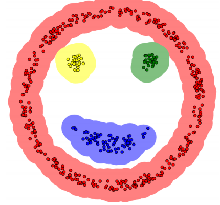
This algorithm divides the region with high enough density into clusters, and can find clusters of any shape

Several concepts

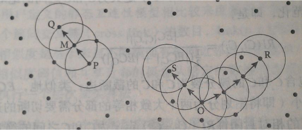
𝛆 neighborhood: the area within the radius 𝜀 of a given object is called the 𝜀 neighborhood of the object.
Core object: if the number of samples in a given neighborhood is greater than or equal to Minpoints, the object is the core object.
Direct density reachable: given an object set D, if p is in the 𝜀 neighborhood of q and q is a core object, we say that the trigger of object p from q is directly density reachable.
Density reachability: set D, there is an object chain p1,p2... pn, p1=q, pn=p,pi+1 is directly reachable from pi about 𝜀 and Minpoints, so point p is reachable from Q about 𝜀 and Minpoints.
Density connection: set D has point o so that points p and q can be reached from the density of O with respect to 𝜀 and Minpoints, then points p and q are connected with respect to the density of 𝜀 and Minpoints.

DBSCAN algorithm idea

1. Specify appropriate 𝜀 and Minpoints.
2. Calculate all sample points. If there are more than Minpoints in the neighborhood of point p, create a new family with p as the core point.
3. Repeatedly look for the points where the direct density of these core points can reach (and then the density can reach), add them to the corresponding clusters, and merge the clusters where the core points are "density connected".
4. When no new points can be added to any cluster, the algorithm ends.

DBSCAN analysis

Disadvantages:
• when the amount of data increases, it requires large memory support and I/O consumption When the density of spatial clustering is uneven and the distance between clusters is very different, the clustering quality is poor.

Comparison between DBSCAN and K-MEANS:

• DBSCAN does not need to enter the number of clusters.
• the shape of the cluster is not required.
• you can enter parameters to filter noise when needed.

code implementation

Case 1
Import package

from sklearn.cluster import DBSCAN
import numpy as np
import pandas as pd
import matplotlib.pyplot as plt

Load data

data = pd.read_csv("kmeans.txt", delimiter=" ")

Training model

# eps distance threshold, min_samples threshold value of the number of samples of the core object in eps field
model = DBSCAN(eps=1.5, min_samples=4)
model.fit(data.iloc[:,:2])

Prediction results

result = model.fit_predict(data.iloc[:,:2])
result

array([ 0, 1, 2, 3, 0, 1, 2, 3, 0, 1, 2, 3, 0, -1, 1, 3, 0,
1, 2, 3, 0, 1, 2, 3, 0, 1, 2, 3, 0, 1, 2, 3, 0, 1,
2, 3, 0, 1, 2, 3, 0, 1, 2, 3, 0, 1, 2, 3, 0, 1, 2,
3, 0, 1, 2, 3, 0, 1, 2, 3, 0, 1, 2, 3, 0, 1, 2, 3,
0, 1, 2, 3, 0, 1, 2, 3, 0, 1, 2], dtype=int64)

Draw a picture to show the clustering results

# Draw each data point and use different colors to represent the classification
mark = ['or', 'ob', 'og', 'oy', 'ok', 'om']
for i in range(len(data)):
    plt.plot(data.iloc[i,0], data.iloc[i,1], mark[result[i]])
    
plt.show()

Case 2
Import package

import numpy as np
import matplotlib.pyplot as plt
from sklearn import datasets

Creating data with datasets

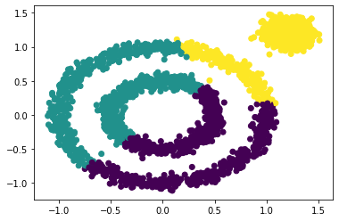
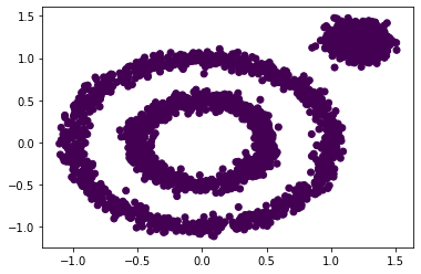
x1, y1 = datasets.make_circles(n_samples=2000, factor=0.5, noise=0.05)
x2, y2 = datasets.make_blobs(n_samples=1000, centers=[[1.2,1.2]], cluster_std=[[.1]])

x = np.concatenate((x1, x2))
plt.scatter(x[:, 0], x[:, 1], marker='o')
plt.show()

x1 is a two-dimensional coordinate, y1 is a list of 0 or 1 (x2,y2 are the same)

Firstly, the kMeans clustering algorithm is established and clustered into three categories

from sklearn.cluster import KMeans
y_pred = KMeans(n_clusters=3).fit_predict(x)
plt.scatter(x[:, 0], x[:, 1], c=y_pred)
plt.show()

Obviously, the result is not good.

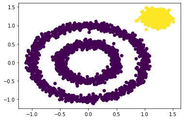
Establish DBSCAN algorithm and adopt default parameters

from sklearn.cluster import DBSCAN
y_pred = DBSCAN().fit_predict(x)
plt.scatter(x[:, 0], x[:, 1], c=y_pred)
plt.show()

By default, the results are grouped into one category, which is different from what you think.

Adjust the value of the parameter eps of DBSCAN

y_pred = DBSCAN(eps = 0.2).fit_predict(x)
plt.scatter(x[:, 0], x[:, 1], c=y_pred)
plt.show()

Adjust the parameters eps and min of DBSCAN_ Value of samples

y_pred = DBSCAN(eps = 0.2, min_samples=50).fit_predict(x)
plt.scatter(x[:, 0], x[:, 1], c=y_pred)
plt.show()

This clustering effect is better than the previous one.