catalogue
General process of decision tree
Write code to calculate empirical entropy
Calculate information gain using code
Select the best data set division method
Differences between ID3, C4.5 and CART
Information gain vs information gain ratio
Visualization of decision tree
Construction of decision tree
The algorithm of decision tree learning is usually a process of recursively selecting the optimal feature and segmenting the training data according to the feature, so that each sub data set has the best classification. This process corresponds to the division of feature space and the construction of decision tree. (1) Start: build the root node, put all training data on the root node, select an optimal feature, and divide the training data set into subsets according to this feature, so that each subset has the best classification under the current conditions.
(2) If these subsets can be classified basically correctly, build leaf nodes and divide these subsets into corresponding leaf nodes.
(3) If there are still subsets that can not be correctly classified, select new optimal features for these subsets, continue to segment them and build corresponding nodes. If recursive, until all training data subsets are basically correctly classified, or there are no appropriate features.
(4) Each subset is divided into leaf nodes, that is, there are clear classes, so a decision tree is generated.
Characteristics of decision tree:
- Advantages: the calculation complexity is not high, the output result is easy to understand, is not sensitive to the loss of intermediate value, and can process irrelevant feature data.
- Disadvantages: over matching may occur
- Applicable data types: numerical type and nominal type
General process of decision tree
First, determine the decisive feature on the current data set. In order to obtain the decisive feature, each feature must be evaluated. After the test is completed, the original data set is divided into several data subsets. These data subsets are distributed on all branches of the first decision point. If the data under a branch belongs to the same type, Then the spam that is currently read out of order has been correctly divided into data categories, and there is no need to further divide the data set. If it does not belong to the same category, it is necessary to divide the data subset repeatedly until all the data of the same type are in one data subset.
The pseudo code createBranch() for creating a branch is shown in the following figure:
If so return Class label:
Else
     Find the best features to divide the dataset
     Partition dataset
     Create branch node
         for Subset of each partition
             Call function createBranch()And add the returned result to the branch node
         return Branch node
The following process is required to make prediction using decision tree:
Collect data: any method can be used. For example, if we want to build a blind date system, we can get data from matchmakers or by visiting blind date objects. According to the factors they consider and the final selection results, we can get some data for us to use.
Data preparation: we should sort out the collected data, sort out all the collected information according to certain rules and typeset it for our subsequent processing.
Analyze data: any method can be used. After the decision tree is constructed, we can check whether the decision tree graph meets the expectations.
Training algorithm: this process is to construct a decision tree. It can also be said that decision tree learning is to construct the data structure of a decision tree.
Test algorithm: use the experience tree to calculate the error rate. When the error rate reaches the acceptable range, the decision tree can be put into use.
Using algorithm: this step can use any supervised learning algorithm, and using decision tree can better understand the internal meaning of data.
information gain
The general principle of data set division is to make disordered data more orderly, but various methods have their own advantages and disadvantages. Information theory is a branch science of quantitative information processing. The change of information before and after data set division is called information gain. The best choice is to obtain the feature with the highest information gain, so we must first learn how to calculate information gain, The measurement of set information is called Shannon entropy, or entropy for short.
Entropy is defined as the expected value of information. If the things to be classified may be divided into multiple classes, the symbol Information defined as:
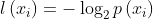
Among them, Is the probability of selecting the classification. In order to calculate entropy, we need to calculate the expected value of information contained in all possible values of all categories, which is obtained by the following formula:
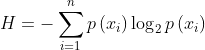
Where N and NN are the number of classifications. The greater the entropy, the greater the uncertainty of random variables.
Information gain: information gain is relative to the feature. Therefore, the information gain g(D,A) of feature A to training data set D is defined as the difference between the empirical entropy H(D) of set D and the empirical conditional entropy H(D|A) of D under the given condition of feature A, that is:
g(D,A)=H(D)−H(D∣A)
Generally, the difference between entropy H(D) and conditional entropy H(D|A) becomes mutual information. The information gain in decision tree learning is equivalent to the mutual information of classes and features in the training data set.
Compared with the training data set, the information gain value has no absolute significance. When the classification problem is difficult, that is, when the empirical entropy of the training data set is large, the information gain value will be too large, on the contrary, the information gain value will be too small. This problem can be corrected by using the information gain ratio, which is another standard for feature selection.
Information gain ratio: the information gain ratio G - R (D, A) of feature A to training data set D is defined as the ratio of its information gain g(D,A) to the empirical entropy of training data set D:
gR(D,A)=H(D)g/(D,A)
Write code to calculate empirical entropy
| ID | time | have the time | Do something meaningful | Is the mood happy | result |
|---|---|---|---|---|---|
| 1 | morning | no | no | commonly | no |
| 2 | morning | no | no | good | no |
| 3 | morning | yes | no | good | yes |
| 4 | morning | yes | yes | commonly | yes |
| 5 | morning | no | no | commonly | no |
| 6 | noon | no | no | commonly | no |
| 7 | noon | no | no | good | no |
| 8 | noon | yes | yes | good | yes |
| 9 | noon | yes | yes | very nice | yes |
| 10 | noon | no | yes | very nice | yes |
| 11 | night | no | yes | very nice | yes |
| 12 | night | no | yes | good | yes |
| 13 | night | yes | no | good | yes |
| 14 | night | yes | no | very nice | yes |
| 15 | night | no | no | commonly | no |
Before writing the code, we annotate the attributes of the dataset.
- Time: 0 for morning, 1 for noon and 2 for evening
- Available time: 0 means no, 1 means yes;
- Do meaningful things: 0 means no, 1 means yes;
- Whether the mood is pleasant: 0 represents general, 1 represents good, and 2 represents very good;
- Results: no stands for no and yes for yes.
Create a dataset and calculate the empirical entropy as follows:
from math import log

"""
Function Description: create test dataset
Parameters: nothing
Returns:
    dataSet: data set
    labels: Classification properties
"""
def creatDataSet():
    # data set
    dataSet=[[0, 0, 0, 0, 'no'],
            [0, 0, 0, 1, 'no'],
            [0, 1, 0, 1, 'yes'],
            [0, 1, 1, 0, 'yes'],
            [0, 0, 0, 0, 'no'],
            [1, 0, 0, 0, 'no'],
            [1, 0, 0, 1, 'no'],
            [1, 1, 1, 1, 'yes'],
            [1, 0, 1, 2, 'yes'],
            [1, 0, 1, 2, 'yes'],
            [2, 0, 1, 2, 'yes'],
            [2, 0, 1, 1, 'yes'],
            [2, 1, 0, 1, 'yes'],
            [2, 1, 0, 2, 'yes'],
            [2, 0, 0, 0, 'no']]
    #Classification properties
    labels=['time','have the time','Do something meaningful','Is the mood happy']
    #Return dataset and classification properties
    return dataSet,labels

"""
Function Description: calculate the empirical entropy (Shannon entropy) of a given data set
Parameters:
    dataSet: data set
Returns:
    shannonEnt: Empirical entropy
"""
def calcShannonEnt(dataSet):
    #Returns the number of rows in the dataset
    numEntries=len(dataSet)
    #Save a dictionary of the number of occurrences of each label
    labelCounts={}
    #Each group of eigenvectors is counted
    for featVec in dataSet:
        currentLabel=featVec[-1]                     #Extract label information
        if currentLabel not in labelCounts.keys():   #If the label is not put into the dictionary of statistical times, add it
            labelCounts[currentLabel]=0
        labelCounts[currentLabel]+=1                 #label count

    shannonEnt=0.0                                   #Empirical entropy
    #Computational empirical entropy
    for key in labelCounts:
        prob=float(labelCounts[key])/numEntries      #Probability of selecting the label
        shannonEnt-=prob*log(prob,2)                 #Calculation by formula
    return shannonEnt                                #Return empirical entropy

#main function
if __name__=='__main__':
    dataSet,features=creatDataSet()
    print(dataSet)
    print(calcShannonEnt(dataSet))
Final results:
The gain of the 0th feature is 0.083
 The gain of the first feature is 0.324
 The gain of the second feature is 0.420
 The gain of the third feature is 0.363
 The gain of the 0th feature is 0.252
 The gain of the first feature is 0.918
 The gain of the second feature is 0.474
{'Do something meaningful': {0: {'have the time': {0: 'no', 1: 'yes'}}, 1: 'yes'}}
Calculate information gain using code
from math import log

"""
Function Description: create test dataset
Parameters: nothing
Returns:
    dataSet: data set
    labels: Classification properties
"""
def creatDataSet():
    # data set
    dataSet=[[0, 0, 0, 0, 'no'],
            [0, 0, 0, 1, 'no'],
            [0, 1, 0, 1, 'yes'],
            [0, 1, 1, 0, 'yes'],
            [0, 0, 0, 0, 'no'],
            [1, 0, 0, 0, 'no'],
            [1, 0, 0, 1, 'no'],
            [1, 1, 1, 1, 'yes'],
            [1, 0, 1, 2, 'yes'],
            [1, 0, 1, 2, 'yes'],
            [2, 0, 1, 2, 'yes'],
            [2, 0, 1, 1, 'yes'],
            [2, 1, 0, 1, 'yes'],
            [2, 1, 0, 2, 'yes'],
            [2, 0, 0, 0, 'no']]
    #Classification properties
    labels=['time','have the time','Do something meaningful','Is the mood happy']
    #Return dataset and classification properties
    return dataSet,labels


"""
Function Description: calculate the empirical entropy (Shannon entropy) of a given data set
Parameters:
    dataSet: data set
Returns:
    shannonEnt: Empirical entropy
"""
def calcShannonEnt(dataSet):
    #Returns the number of rows in the dataset
    numEntries=len(dataSet)
    #Save a dictionary of the number of occurrences of each label
    labelCounts={}
    #Each group of eigenvectors is counted
    for featVec in dataSet:
        currentLabel=featVec[-1]                     #Extract label information
        if currentLabel not in labelCounts.keys():   #If the label is not put into the dictionary of statistical times, add it
            labelCounts[currentLabel]=0
        labelCounts[currentLabel]+=1                 #label count

    shannonEnt=0.0                                   #Empirical entropy
    #Computational empirical entropy
    for key in labelCounts:
        prob=float(labelCounts[key])/numEntries      #Probability of selecting the label
        shannonEnt-=prob*log(prob,2)                 #Calculation by formula
    return shannonEnt                                #Return empirical entropy


"""
Function Description: calculate the empirical entropy (Shannon entropy) of a given data set
Parameters:
    dataSet: data set
Returns:
    shannonEnt: Index value of maximum information gain feature
"""
def chooseBestFeatureToSplit(dataSet):
    #Number of features
    numFeatures = len(dataSet[0]) - 1
    #Shannon entropy of counting data set
    baseEntropy = calcShannonEnt(dataSet)
    #information gain
    bestInfoGain = 0.0
    #Index value of optimal feature
    bestFeature = -1
    #Traverse all features
    for i in range(numFeatures):
        # Get the i th all features of dataSet
        featList = [example[i] for example in dataSet]
        #Create set set {}, elements cannot be repeated
        uniqueVals = set(featList)
        #Empirical conditional entropy
        newEntropy = 0.0
        #Calculate information gain
        for value in uniqueVals:
            #The subset of the subDataSet after partition
            subDataSet = splitDataSet(dataSet, i, value)
            #Calculate the probability of subsets
            prob = len(subDataSet) / float(len(dataSet))
            #The empirical conditional entropy is calculated according to the formula
            newEntropy += prob * calcShannonEnt((subDataSet))
        #information gain
        infoGain = baseEntropy - newEntropy
        #Print information gain for each feature
        print("The first%d The gain of each feature is%.3f" % (i, infoGain))
        #Calculate information gain
        if (infoGain > bestInfoGain):
            #Update the information gain to find the maximum information gain
            bestInfoGain = infoGain
            #Record the index value of the feature with the largest information gain
            bestFeature = i
            #Returns the index value of the feature with the maximum information gain
    return bestFeature

"""
Function Description: divide the data set according to the given characteristics
Parameters:
    dataSet: Data set to be divided
    axis: Characteristics of partitioned data sets
    value: The value of the feature to be returned
Returns:
    shannonEnt: Empirical entropy
"""
def splitDataSet(dataSet,axis,value):
    retDataSet=[]
    for featVec in dataSet:
        if featVec[axis]==value:
            reducedFeatVec=featVec[:axis]
            reducedFeatVec.extend(featVec[axis+1:])
            retDataSet.append(reducedFeatVec)
    return retDataSet


#main function
if __name__=='__main__':
    dataSet,features=creatDataSet()
    # print(dataSet)
    # print(calcShannonEnt(dataSet))
    print("Optimal index value:"+str(chooseBestFeatureToSplit(dataSet)))
Final result:
The gain of the 0th feature is 0.083
 The gain of the first feature is 0.324
 The gain of the second feature is 0.420
 The gain of the third feature is 0.363
 Optimal index value: 2
Compare our own calculation results and find that the results are correct! The index value of the optimal feature is 2, that is, feature A3 (doing meaningful things).
Partition dataset
In addition to measuring the information entropy, the classification algorithm also needs to divide the data set and measure the entropy of the divided data set, so as to judge whether the data set is divided correctly:
# Code function: dividing data sets
def splitDataSet(dataSet,axis,value): #Pass in three parameters: the dataset to be divided, the characteristics of the dataset to be divided, and the value of the characteristics to be returned
    retDataSet = [] #As the linked list dataSet of the parameter, we get its address, that is, reference. Direct operation on the linked list will change its value, so we create a new linked list to operate

    for featVec in dataSet:
        if featVec[axis] == value: #If a feature is equal to the feature value we specify
        #Remove this feature and create a sub feature
            reduceFeatVec = featVec[:axis]
            reduceFeatVec.extend(featVec[axis+1:])
            #Add the qualified samples and the cut samples to our newly established samples
            retDataSet.append(reduceFeatVec)

    return retDataSet
Select the best data set division method
def chooseBestFeatureToSplit(dataSet):
	# Obtain the feature number of a sample in our sample set (because the feature number of each sample is the same, which is equivalent to the number of all features we can use as the classification basis). The last column of our sample is the category to which the sample belongs, so to subtract the category information, in our example, the feature number is 2
    numFeatures = len(dataSet[0])-1
    #Calculate the initial Shannon entropy of the sample
    baseEntropy = calcShannonEnt(dataSet)
    #Initialize maximum information gain
    bestInfoGain =0.0
    #Optimal partition feature
    bestFeature = -1

    for i in range(numFeatures):
        featList = [sample[i] for sample in dataSet] # We first traverse the entire data set, get the possible value of the first eigenvalue, and then assign it to a linked list. Our first eigenvalue value is [1,1,1,0,0], in fact, there are only two values of [1,0]
        uniqueVals = set(featList)
        newEntropy = 0.0
        for value in uniqueVals: #uniqueVals stores the possibility of all values of the eigenvalues of a sample
            subDataSet = splitDataSet(dataSet,i,value)
            prob = len(subDataSet)/float(len(dataSet))
            newEntropy += prob * calcShannonEnt(subDataSet)

        infoGain = baseEntropy - newEntropy# Calculate the information gain

        if(infoGain > bestInfoGain):
            bestInfoGain = infoGain
            bestFeature = i

    return bestFeature
Information gain rate
In view of the lack of information gain, we hope to make some adjustments to the calculation of information gain, that is, when there are many kinds of eigenvalues, its importance will be greatly reduced. The adjusted information gain is called information gain rate.
Gain rate: gain rate is defined by the ratio of Gain(D, a) and intrinsic value corresponding to attribute a.
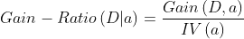
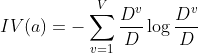
- Gain_Ratio indicates information gain rate
- IV represents the information entropy of the feature
- Feature information gain ➗ Information entropy of feature
a. If there are many kinds of eigenvalues of a feature, the greater the information entropy, that is, the more kinds of eigenvalues, the greater the coefficient divided by.
b. If the type of eigenvalue of a feature is small, the smaller its information entropy is, that is, the smaller the type of eigenvalue, the smaller the coefficient divided by.
Gini coefficient
Gini coefficient: indicates the probability that a randomly selected sample in the sample set will be misdivided
Gini coefficient = probability that the sample is selected * probability that the sample is misclassified
Gini coefficient has the same properties as information entropy: it measures the uncertainty of random variables;
The greater the G, the higher the uncertainty of the data;
The smaller the G, the lower the uncertainty of the data;
G = 0, all samples in the dataset are of the same category;
In the classification problem, assuming that D has k classes and the probability that the sample point belongs to class k is pk, the Gini value of the probability distribution is defined as: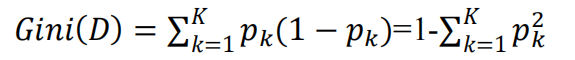
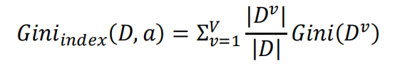
Given dataset D, the Gini index of attribute a is defined as:
Differences between ID3, C4.5 and CART
1, ID3
Entropy represents the amount of information contained in the data. The smaller the entropy, the higher the purity of the data, that is, the more consistent the data is. This is what we want each child node to look like after division.
Information gain = pre partition entropy - post partition entropy. The greater the information gain, the greater the "purity improvement" obtained by using attribute a to partition * *. That is, the higher the purity of the results obtained by using attribute a to partition the training set.
ID3 is only applicable to binary classification problems. ID3 can only deal with discrete attributes.
2, C4.5
C4.5 overcomes the problem that ID3 can only deal with discrete attributes and the problem that information gain tends to select features with more values, and uses information gain ratio to select features. Information gain ratio = information gain / entropy before division, and selects the feature with the largest information gain ratio as the optimal feature.
C4.5 when dealing with continuous features, the feature values are sorted first, and the intermediate value of two consecutive values is used as the division standard. Try each partition, calculate the corrected information gain, and select the split point with the largest information gain as the split point of the attribute.
3, CART
CART differs from ID3 and C4.5 in that the tree generated by CART must be a binary tree. In other words, whether it is a regression or classification problem, whether the feature is discrete or continuous, whether there are multiple or two attribute values, the internal node can only be divided according to the attribute value.
The full name of CART is classification and regression tree. From this name, we should know that CART can be used not only for classification problems, but also for regression problems.
In the regression tree, the square error minimization criterion is used to select features and divide them. The predicted value given by each leaf node is the mean of all sample target values divided into the leaf node, which only minimizes the square error under the given division.
To determine the optimal score, we also need to traverse all attributes and all their values to try to divide them respectively, calculate the minimum square error in this case, and select the smallest as the basis for this division. Because the least square error minimization criterion is used in the generation of regression tree, it is also called least square regression tree.
Classify tree species, and use Gini index minimization criterion to select features and divide them;
The Gini index represents the uncertainty, or impure, of the set. The greater the Gini index, the higher the uncertainty of the set and the greater the purity. This is similar to entropy. Another way to understand Gini index is that Gini index is to minimize the probability of misclassification.
Information gain vs information gain ratio
The reason why information gain ratio is introduced is due to a disadvantage of information gain. That is: information gain always tends to select attributes with more values. A penalty term is added to the information gain ratio to solve this problem.
gini index vs entropy
- The calculation of Gini index does not need logarithmic operation, which is more efficient;
- Gini index is more inclined to continuous attributes, and entropy is more inclined to discrete attributes.
Visualization of decision tree
The realization of decision tree visualization is realized by using the code in Matplotlib
from math import log
import operator
from matplotlib.font_manager import FontProperties
import matplotlib.pyplot as plt
"""
Function Description: get the number of leaf nodes of the decision tree

Parameters:
    myTree: Decision tree
Returns:
    numLeafs: Number of leaf nodes of the decision tree
"""
def getNumLeafs(myTree):
    numLeafs=0
    firstStr=next(iter(myTree))
    secondDict=myTree[firstStr]
    for key in secondDict.keys():
        if type(secondDict[key]).__name__=='dict':
            numLeafs+=getNumLeafs(secondDict[key])
        else: numLeafs+=1
    return numLeafs

"""
Function description:Gets the number of layers of the decision tree

Parameters:
    myTree:Decision tree
Returns:
    maxDepth:Layers of decision tree
"""
def getTreeDepth(myTree):
    maxDepth = 0                                                #Initialize decision tree depth
    firstStr = next(iter(myTree))                                #myTree.keys() in Python 3 returns dict_keys is no longer a list, so you can't use the method of myTree.keys()[0] to obtain node properties. You can use list(myTree.keys())[0]
    secondDict = myTree[firstStr]                                #Get next dictionary
    for key in secondDict.keys():
        if type(secondDict[key]).__name__=='dict':                #Test whether the node is a dictionary. If it is not a dictionary, it means that the node is a leaf node
            thisDepth = 1 + getTreeDepth(secondDict[key])
        else:   thisDepth = 1
        if thisDepth > maxDepth: maxDepth = thisDepth            #Update layers
    return maxDepth

"""
Function description:Draw node

Parameters:
    nodeTxt - Node name
    centerPt - Text position
    parentPt - Arrow position of dimension
    nodeType - Node format
Returns:
    nothing
"""
def plotNode(nodeTxt, centerPt, parentPt, nodeType):
    arrow_args = dict(arrowstyle="<-")                                            #Define arrow format
    font = FontProperties(fname=r"c:\windows\fonts\simsun.ttc", size=14)        #Set Chinese font
    createPlot.ax1.annotate(nodeTxt, xy=parentPt,  xycoords='axes fraction',    #Draw node
        xytext=centerPt, textcoords='axes fraction',
        va="center", ha="center", bbox=nodeType, arrowprops=arrow_args, FontProperties=font)

"""
Function description:Dimension directed edge attribute values

Parameters:
    cntrPt,parentPt - Used to calculate dimension locations
    txtString - Marked content
Returns:
    nothing
"""
def plotMidText(cntrPt, parentPt, txtString):
    xMid = (parentPt[0]-cntrPt[0])/2.0 + cntrPt[0]                                            #Calculate dimension location
    yMid = (parentPt[1]-cntrPt[1])/2.0 + cntrPt[1]
    createPlot.ax1.text(xMid, yMid, txtString, va="center", ha="center", rotation=30)

"""
Function description:Draw decision tree

Parameters:
    myTree - Decision tree(Dictionaries)
    parentPt - Marked content
    nodeTxt - Node name
Returns:
    nothing
"""
def plotTree(myTree, parentPt, nodeTxt):
    decisionNode = dict(boxstyle="sawtooth", fc="0.8")                                        #Set node format
    leafNode = dict(boxstyle="round4", fc="0.8")                                            #Format leaf nodes
    numLeafs = getNumLeafs(myTree)                                                          #Get the number of decision leaf nodes, which determines the width of the tree
    depth = getTreeDepth(myTree)                                                            #Get the number of decision tree layers
    firstStr = next(iter(myTree))                                                            #Next dictionary
    cntrPt = (plotTree.xOff + (1.0 + float(numLeafs))/2.0/plotTree.totalW, plotTree.yOff)    #Center position
    plotMidText(cntrPt, parentPt, nodeTxt)                                                    #Dimension directed edge attribute values
    plotNode(firstStr, cntrPt, parentPt, decisionNode)                                        #Draw node
    secondDict = myTree[firstStr]                                                            #The next dictionary is to continue drawing child nodes
    plotTree.yOff = plotTree.yOff - 1.0/plotTree.totalD                                        #y offset
    for key in secondDict.keys():
        if type(secondDict[key]).__name__=='dict':                                            #Test whether the node is a dictionary. If it is not a dictionary, it means that the node is a leaf node
            plotTree(secondDict[key],cntrPt,str(key))                                        #It is not a leaf node, and the recursive call continues to draw
        else:                                                                                #If it is a leaf node, draw the leaf node and mark the directed edge attribute value
            plotTree.xOff = plotTree.xOff + 1.0/plotTree.totalW
            plotNode(secondDict[key], (plotTree.xOff, plotTree.yOff), cntrPt, leafNode)
            plotMidText((plotTree.xOff, plotTree.yOff), cntrPt, str(key))
    plotTree.yOff = plotTree.yOff + 1.0/plotTree.totalD

"""
Function description:Create a paint panel

Parameters:
    inTree - Decision tree(Dictionaries)
Returns:
    nothing
"""
def createPlot(inTree):
    fig = plt.figure(1, facecolor='white')#Create fig
    fig.clf()#Empty fig
    axprops = dict(xticks=[], yticks=[])
    createPlot.ax1 = plt.subplot(111, frameon=False, **axprops)#Remove the x and y axes
    plotTree.totalW = float(getNumLeafs(inTree))#Get the number of decision nodes
    plotTree.totalD = float(getTreeDepth(inTree))#Get the number of decision tree layers
    plotTree.xOff = -0.5/plotTree.totalW; plotTree.yOff = 1.0#x offset
    plotTree(inTree, (0.5,1.0), '')#Draw decision tree
    plt.show()#Display drawing results

if __name__ == '__main__':
    dataSet, labels = createDataSet()
    featLabels = []
    myTree = createTree(dataSet, labels, featLabels)
    print(myTree)
    createPlot(myTree)

if __name__=='__main__':
    dataSet,labels=createDataSet()
    featLabels=[]
    myTree=createTree(dataSet,labels,featLabels)
    print(myTree)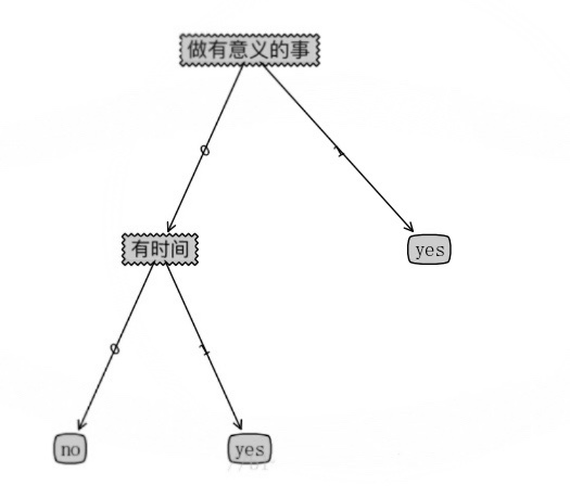
summary
The decision tree algorithm mainly includes three parts: feature selection, tree generation and tree pruning. Common algorithms include ID3, C4.5 and CART. Generation of decision tree. Usually, the maximum information gain, the maximum information gain ratio and the minimum Gini index are used as the criteria of feature selection. Starting from the root node, the decision tree is generated recursively. It is equivalent to continuously selecting local optimal features, or dividing the training set into subsets that can basically be classified correctly. Decision tree learning may create an overly complex tree and can not predict data well. That is, over fitting. The pruning mechanism (not supported at present) can avoid over fitting by setting the minimum number of samples or the maximum depth of a leaf node. The traditional decision tree algorithm is based on heuristic algorithms, such as greedy algorithm, that is, each node creates the optimal decision. These algorithms cannot produce an optimal decision tree. Random sampling of samples and features can reduce the overall effect deviation.