This course is the after-school code of the "dimension reduction" chapter of machine learning. Course address: https://www.icourse163.org/course/WZU-1464096179 Course complete code: https://github.com/fengdu78/WZU-machine-learning-course Code modification and comment: Huang haiguang, haiguang2000@wzu.edu.cn

Principal component analysis

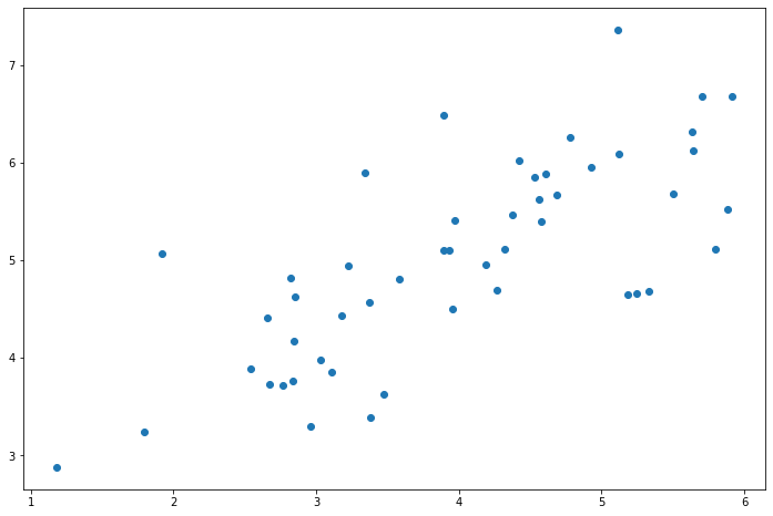
PCA is a linear transformation to find the "principal component" or the direction of maximum variance in the data set. It can be used for dimensionality reduction. In this exercise, we are first responsible for implementing PCA and applying it to a simple two-dimensional dataset to understand how it works. Let's start by loading and visualizing datasets.

import numpy as np
import pandas as pd
import matplotlib.pyplot as plt
import seaborn as sb
from scipy.io import loadmat

data = pd.read_csv('data/pcadata.csv')
data.head()

X = data.values

fig, ax = plt.subplots(figsize=(12,8))
ax.scatter(X[:, 0], X[:, 1])
plt.show()

PCA algorithm is quite simple. After ensuring that the data is normalized, the output is only the singular value decomposition of the covariance matrix of the original data.

def pca(X):
    # normalize the features
    X = (X - X.mean()) / X.std()

    # compute the covariance matrix
    X = np.matrix(X)
    cov = (X.T * X) / X.shape[0]

    # perform SVD
    U, S, V = np.linalg.svd(cov)

    return U, S, V

U, S, V = pca(X)
U, S, V

(matrix([[-0.79241747, -0.60997914],
         [-0.60997914,  0.79241747]]),
 array([1.43584536, 0.56415464]),
 matrix([[-0.79241747, -0.60997914],
         [-0.60997914,  0.79241747]]))

Now we have principal components (matrix U), which we can use to project the original data into a lower dimensional space. For this task, we will implement a function that calculates the projection and selects only the top K components, which effectively reduces the dimension.

def project_data(X, U, k):
    U_reduced = U[:,:k]
    return np.dot(X, U_reduced)

Z = project_data(X, U, 1)

We can also restore the original data through the reverse conversion step.

def recover_data(Z, U, k):
    U_reduced = U[:,:k]
    return np.dot(Z, U_reduced.T)

X_recovered = recover_data(Z, U, 1)

fig, ax = plt.subplots(figsize=(12,8))
ax.scatter(list(X_recovered[:, 0]), list(X_recovered[:, 1]))
plt.show()

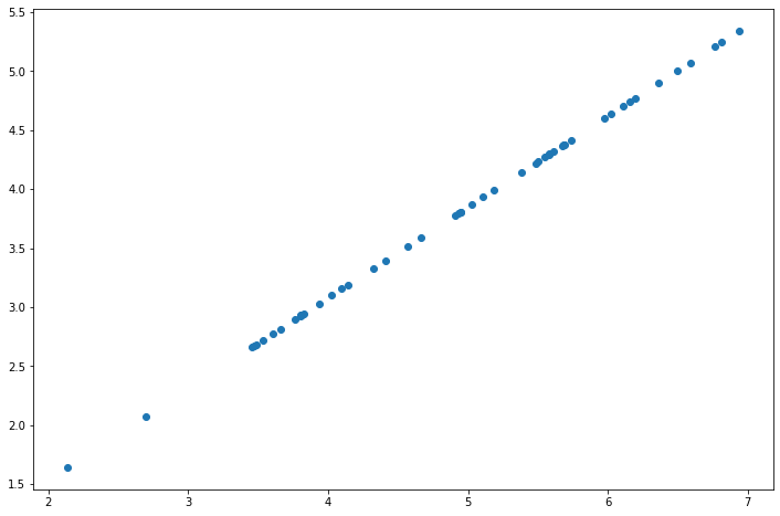
Note that the projection axis of the first principal component is basically a diagonal in the dataset. When we reduce the data to one dimension, we lose the changes around the diagonal, so in our reproduction, everything follows the diagonal.

Our last task in this exercise is to apply PCA to face images. By using the same dimensionality reduction technology, we can capture the "essence" of the image with much less data than the original image.

faces = loadmat('data/ex7faces.mat')
X = faces['X']
X.shape

(5000, 1024)

def plot_n_image(X, n):
    """ plot first n images
    n has to be a square number
    """
    pic_size = int(np.sqrt(X.shape[1]))
    grid_size = int(np.sqrt(n))

    first_n_images = X[:n, :]

    fig, ax_array = plt.subplots(nrows=grid_size,
                                 ncols=grid_size,
                                 sharey=True,
                                 sharex=True,
                                 figsize=(8, 8))

    for r in range(grid_size):
        for c in range(grid_size):
            ax_array[r, c].imshow(first_n_images[grid_size * r + c].reshape(
                (pic_size, pic_size)))
            plt.xticks(np.array([]))
            plt.yticks(np.array([]))

The exercise code includes a function that renders the first 100 faces in the dataset. Instead of trying to regenerate here, you can see what they look like in the exercise text. We can easily render at least one image.

face = np.reshape(X[3,:], (32, 32))

plt.imshow(face)
plt.show()

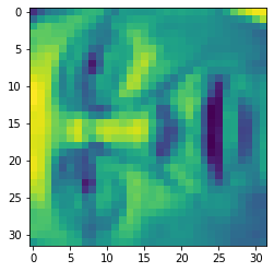
It looks terrible. These images are only 32 x 32 grayscale (it is also side rendering, but we can ignore it now). Our next step is to run PCA on the face dataset and obtain the first 100 main features.

U, S, V = pca(X)
Z = project_data(X, U, 100)

Now we can try to restore the original structure and render again.

X_recovered = recover_data(Z, U, 100)
face = np.reshape(X_recovered[3,:], (32, 32))
plt.imshow(face)
plt.show()

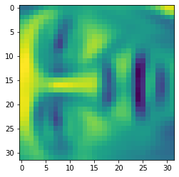
We can see that the data dimension is reduced, but the details are not lost.

reference resources

• Prof. Andrew Ng. Machine Learning. Stanford University