1. Introduction to algorithm

        The working principle of k-nearest neighbor algorithm is that there is a sample data set, also known as training sample set, and each data in the sample set has a label, that is, we know the corresponding relationship between each data in the sample set and its classification. After entering the new data without labels, each feature of the new data is compared with the corresponding feature of the data in the sample set, and then the algorithm extracts the classification label of the data with the most similar feature (nearest neighbor) in the sample set. Generally speaking, we only select the first k most similar data in the sample data set, which is the source of K in the k-nearest neighbor algorithm. Generally, K is an integer not greater than 20. Finally, select the classification that appears most in the k most similar data as the classification of new data.

          Advantages: high precision, insensitive to outliers and no data input assumption.                                                                           Disadvantages: high computational complexity and space complexity.                                                                                                 Applicable data range: numerical type and standard type.

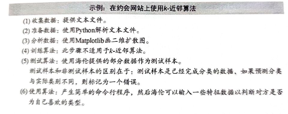
         The general flow of k-nearest neighbor algorithm is shown in the book:

2. Examples

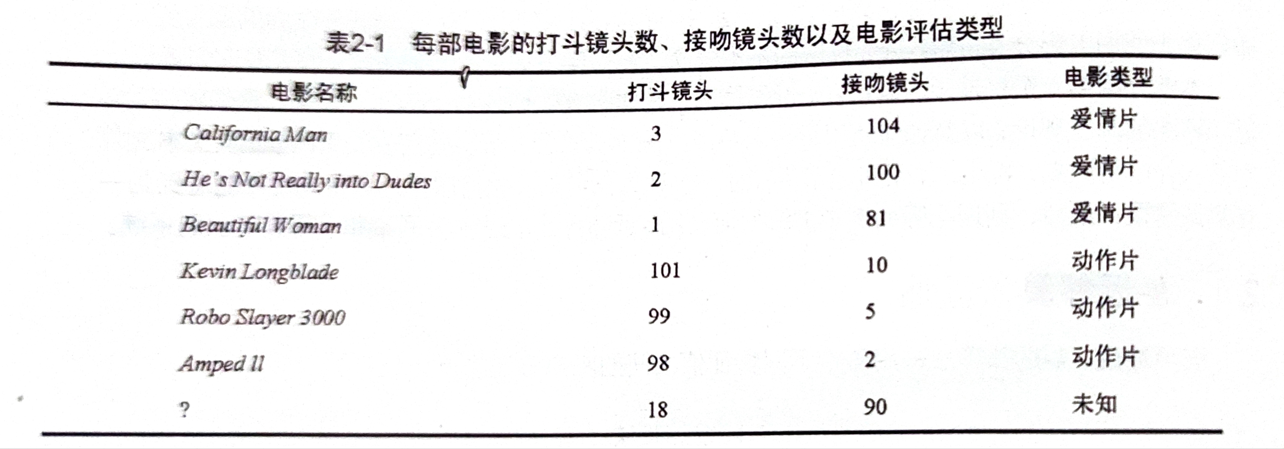
        Taking film classification as an example, kNN can be used to classify whether a film is a love film or an action film.

 

          The above figure is a data set, that is, a training sample set. Generally speaking, we divide kissing scenes into romantic films. There are many fighting scenes, which are divided into action films. According to the data of the original six films, even if we don't know what type of unknown films belong to, we can judge by calculating the distance from these films.

          In the figure above, we get the distance between the film in the sample and the unknown film. Assuming k=3, the three closest to the unknown film are all love films, so we judge the unknown film as a love film.

3. Code implementation

        Take improving dating website pairing as an example

Preparing data: parsing data from a text file

         Resolver for converting text records to NumPy

def file2matrix(filename):
    # Open file
    fr = open(filename)
    # Read all contents of the file
    arrayOlines = fr.readlines()
    # Get the number of file lines
    numberOfLines = len(arrayOlines)
    # Returned NumPy matrix numberOfLines row, 3 columns
    returnMat = np.zeros((numberOfLines, 3))
    # Create category label vector
    classLabelVector = []
    # Index value of row
    index = 0
    # Read each line
    for line in arrayOlines:
        # Remove the white space at the beginning and end of each line, such as' \ n','\r','\t ','
        line = line.strip()
        # Slice the contents of each row according to the '\ t' symbol. In this example, there are four columns
        listFromLine = line.split('\t')
        # The first three columns of data are extracted and stored in the returnMat matrix, that is, the characteristic matrix
        returnMat[index, :] = listFromLine[0:3]  # Put in the index line of returnMat
        # Classification according to text content 1: dislike; 2: General; 3: Like
        if listFromLine[-1] == 'didntLike':
            classLabelVector.append(1)
        elif listFromLine[-1] == 'smallDoses':
            classLabelVector.append(2)
        elif listFromLine[-1] == 'largeDoses':
            classLabelVector.append(3)
        index += 1
    # Returns the label column vector and the characteristic matrix
    return returnMat, classLabelVector

Analyzing data: creating scatter charts using Matplotlib

import matplotlib
import matplotlib.pyplot as plt
fig = plt.figure()
ax = fig.add_subplot(111)
ax.scatter(datingDataMat[:, 1], datingDataMat[:, 2], 
15.0*array(datingLabels), 15.0*array(datingLabels))
plt.show()

Prepare data: normalized value

        Normalized eigenvalue

def autoNorm(dataSet):
    # Gets the minimum value of the data
    minVals = dataSet.min(0)
    # Gets the maximum value of the data
    maxVals = dataSet.max(0)
    # Range of maximum and minimum values
    ranges = maxVals - minVals
    # shape(dataSet) returns the number of matrix rows and columns of the dataSet
    normDataSet = np.zeros(np.shape(dataSet))
    # numpy function shape[0] returns the number of rows of dataSet
    m = dataSet.shape[0]
    # Original value minus minimum value (x-xmin)
    normDataSet = dataSet - np.tile(minVals, (m, 1))
    # Difference divided by the difference between maximum and minimum (x-xmin) / (xmax xmin)
    normDataSet = normDataSet / np.tile(ranges, (m, 1))
    # Normalized data results, data range, minimum
    return normDataSet, ranges, minVals

Test algorithm: verify the classifier as a complete program

        Classifier test code for dating website

def datingClassTest():
    # Open file name
    filename = "datingTestSet.txt"
    # Store the returned feature matrix and classification vector in datingDataMat and datingLabels respectively
    datingDataMat, datingLabels = file2matrix(filename)
    # Take 10% of all data. The smaller the Horatio, the lower the error rate
    hoRatio = 0.10
    # Data normalization, return normalized data result, data range, minimum value
    normMat, ranges, minVals = autoNorm(datingDataMat)
    # Gets the number of rows of normMat
    m = normMat.shape[0]
    # 10% number of test data
    numTestVecs = int(m * hoRatio)
    # Classification error count
    errorCount = 0.0
    for i in range(numTestVecs):
        # The first numTestVecs data is used as the test set, and the last m-numTestVecs data is used as the training set
        # k select the number of label s + 1 (the result is better)
        classifierResult = classify0(normMat[i, :], normMat[numTestVecs:m, :], \
                                     datingLabels[numTestVecs:m], 4)
        print("Classification results:%d\t Real category:%d" % (classifierResult, datingLabels[i]))
        if classifierResult != datingLabels[i]:
            errorCount += 1.0
    print("error rate:%f%%" % (errorCount / float(numTestVecs) * 100))

Using algorithms: building complete and usable systems

        Dating site prediction function

       

def classifyPerson():
    # Output results
    resultList = ['Detestable', 'Some like', 'like it very much']
    # 3D feature user input
    percentTats = float(input("Percentage of time spent playing video games:"))
    ffMiles = float(input("Frequent flyer miles obtained each year:"))
    iceCream = float(input("Litres of ice cream consumed per week:"))
    # Open file name
    filename = "datingTestSet.txt"
    # Open and process data
    datingDataMat, datingLabels = file2matrix(filename)
    # Training set normalization
    normMat, ranges, minVals = autoNorm(datingDataMat)
    # Generate NumPy array, test set
    inArr = np.array([percentTats, ffMiles, iceCream])
    # Test set normalization
    norminArr = (inArr - minVals) / ranges
    # Return classification results
    classifierResult = classify0(norminArr, normMat, datingLabels, 4)
    # Print results
    print("You may%s this man" % (resultList[classifierResult - 1]))

4. Summary

         K-NN is a case-based learning, or local approximation and lazy learning that postpones all calculations until after classification. k-nearest neighbor algorithm is one of the simplest machine learning algorithms.