task

A handwritten numeral classifier is trained using MNIST data set.

Prepare dataset

The data set is an array of 70000784, 70000 pictures, each with 728 pixels, which can be displayed by resizing into 2828 pictures. All the training processes here use a 728 length vector. However, it can be seen that this method is obviously not well applied to the two-dimensional information of the image, which is why the convolutional neural network works well.

# The old version used mnist = fetch_mldata('MNIST original')
from sklearn.datasets import fetch_openml
mnist = fetch_openml('MNIST_784')
X, y = mnist["data"], mnist["target"]
X_train, X_test, y_train, y_test = X[:60000], X[60000:], y[:60000], y[60000:]
-----------------------------
mnist['data'] #Training set 70000 * 78470000 black and white images, one size 28 * 28
mnist['target'] #['1', '3', '4'...] label

Training a binary classifier

A simple linear model and random gradient descent are used to train a model to judge whether it is 5 or not

import numpy as np
# Disorder order
shuffle_index = np.random.permutation(60000)
X_train, y_train = X_train[shuffle_index], y_train[shuffle_index]
# Two classifier
y_train_5 = (y_train == '5') # True for all 5s, False for all other digits.
y_test_5 = (y_test == '5')
# To classify with linear model is to classify with quadratic form
from sklearn.linear_model import SGDClassifier
sgd_clf = SGDClassifier(random_state=42)
sgd_clf.fit(X_train, y_train_5)
sgd_clf.predict([50])

Performance evaluation

• Cross validation
  The most basic cross validation, "accuracy" is the accuracy rate, and the correct proportion of all predictions. The problem with this evaluation method is that if I guess all the answers are not 5, there will be 90% accuracy, so we need a better evaluation method

# Cross validation
from sklearn.model_selection import cross_val_score
# Classification problem, using accuracy accuracy as score
scores = cross_val_score(sgd_clf,X_train,y_train_5,scoring="accuracy", cv=3)
scores

• Accuracy
  That is, the correct proportion is detected in all samples detected as target objects
• recall
  Is the proportion of all targets detected

from sklearn.metrics import precision_score, recall_score
print(precision_score(y_train_5, y_train_pred)) #Accuracy, the proportion found in all 5
recall_score(y_train_5, y_train_pred)  #Recall rate, all considered 5, the proportion of 5

• Obviously, we want both accuracy and recall to be high, but the relationship between them presents a seesaw relationship

y_scores = cross_val_predict(sgd_clf, X_train, y_train_5, cv=3,
method="decision_function")
from sklearn.metrics import precision_recall_curve
precisions, recalls, thresholds = precision_recall_curve(y_train_5, y_scores)
def plot_precision_recall_vs_threshold(precisions, recalls, thresholds):
    plt.plot(thresholds, precisions[:-1], "b--", label="Precision")
    plt.plot(thresholds, recalls[:-1], "g-", label="Recall")
    plt.xlabel("Threshold")
    plt.legend(loc="upper left")
    plt.ylim([0, 1])
plot_precision_recall_vs_threshold(precisions, recalls, thresholds)

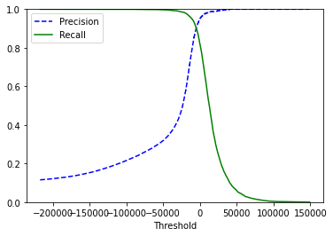
Therefore, we need to select an appropriate threshold (the threshold can be obtained by using precision_recall_curve, that is, the credibility of the structure). Sometimes we want high accuracy (such as face recognition), and sometimes we want high recall rate (such as quality inspection, we'd rather check more than Miss)

• PR curve
  The curve of accuracy and recall should be as close to the upper right corner as possible

plt.plot(precisions,recalls)

• F1 score
  The harmonic average of recall and accuracy can be used as the detection score

from sklearn.metrics import f1_score
f1_score(y_train_5, y_train_pred)

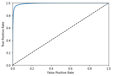
• ROC curve
  FPR is the rate at which negative examples are erroneously divided into positive examples
  TNR is the rate at which counterexamples are correctly classified
  It should be as close to the upper left corner as possible
  Use the PR curve first when there are few positive examples, or when you pay more attention to false positive examples than false negative examples (you'd rather kill one by mistake). ROC curve is used in other cases.

from sklearn.metrics import roc_curve
fpr, tpr, thresholds = roc_curve(y_train_5, y_scores)
def plot_roc_curve(fpr, tpr, label=None):
    plt.plot(fpr, tpr, linewidth=2, label=label)
    plt.plot([0, 1], [0, 1], 'k--')
    plt.axis([0, 1, 0, 1])
    plt.xlabel('False Positive Rate')
    plt.ylabel('True Positive Rate')
plot_roc_curve(fpr, tpr, None)
from sklearn.metrics import roc_auc_score
roc_auc_score(y_train_5, y_scores)

Multi classification problem

Some algorithms (such as random forest classifier or naive Bayesian classifier) can directly deal with multi class classification problems. Other algorithms (such as SVM classifier or linear classifier) are strict binary classifiers. Then, there are many strategies that allow you to use two classifiers to perform multi class classification.
One strategy is to train a binary classification for each, and then see which is the most reliable. OvA
The other is to train a two category for every two, and then compete. A lot of classifiers need to be trained. OvO
Some algorithms (such as SVM classifier) are difficult to expand in the size of the training set, so OvO is better for these algorithms, because it can train more on small data sets than on huge data sets. However, for most binary classifiers, OvA is a better choice.

Let's train any one, except SVM, which is OVA by default

sgd_clf.fit(X_train, y_train) # y_train, not y_train_5

You can also force the use of ovo or ova policies

from sklearn.multiclass import OneVsOneClassifier
ovo_clf = OneVsOneClassifier(SGDClassifier(random_state=42))
ovo_clf.fit(X_train, y_train)
len(ovo_clf.estimators_)

There is no problem of ova or ovo in the multi classifier of random forest

Error analysis of multi classification problem

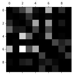
Confusion matrix a [i] [j], the number of classes I divided into j

from sklearn.preprocessing import StandardScaler
scaler = StandardScaler()
X_train_scaled = scaler.fit_transform(X_train.astype(np.float64)) #Simple regularization
y_train_pred = cross_val_predict(sgd_clf, X_train_scaled, y_train, cv=3)
conf_mx = confusion_matrix(y_train, y_train_pred)
plt.matshow(conf_mx, cmap=plt.cm.gray)
plt.show()

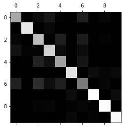
It can be seen from this picture that the classifier works well, but we need to deal with it a little if we want to see more useful data.
First divide each value of the confusion matrix by the total number of corresponding categories, and then fill the diagonal with 0 (because the diagonal number is too large)

row_sums = conf_mx.sum(axis=1, keepdims=True)
norm_conf_mx = conf_mx / row_sums
np.fill_diagonal(norm_conf_mx, 0)
plt.matshow(norm_conf_mx, cmap=plt.cm.gray)
plt.show()

You can see which numbers are easily misclassified

• Special case analysis: we can take out the wrong numbers separately to analyze which cases will be wrong. Can we add this feature through some means so that the training can distinguish these cases.

Multi label classification

A picture may have many labels. A classifier is trained to recognize three faces, Alice, Bob and Charlie; Then when it is input a picture containing Alice and Bob, it should output [1, 0, 1]

from sklearn.neighbors import KNeighborsClassifier
y_train_large = (y_train >= 7)
y_train_odd = (y_train % 2 == 1)
y_multilabel = np.c_[y_train_large, y_train_odd]
knn_clf = KNeighborsClassifier()
knn_clf.fit(X_train, y_multilabel)
knn_clf.predict([some_digit])

That is, the tag becomes a multivariable array, and the others remain unchanged

We use the average value of F1 as the evaluation score, or use the weighted average value (number of tags), average = "weighted".

y_train_knn_pred = cross_val_predict(knn_clf, X_train, y_train, cv=3)
f1_score(y_train, y_train_knn_pred, average="macro")
y_train_knn_pred = cross_val_predict(knn_clf, X_train, y_train, cv=3)
f1_score(y_train, y_train_knn_pred, average="weighted")

Multiple output classification

Generalization of multi label problem, each label has multiple values
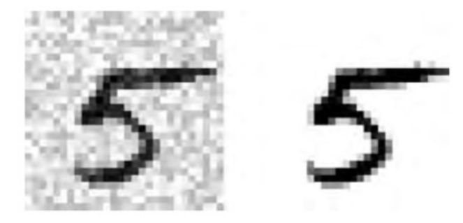
For example, input a noisy image and output a clean image. Each point is a class with 0-255 values

import random as rnd
noise = rnd.randint(0, 100, (len(X_train), 784))
noise = rnd.randint(0, 100, (len(X_test), 784))
X_train_mod = X_train + noise
X_test_mod = X_test + noise
y_train_mod = X_train
y_test_mod = X_test
knn_clf.fit(X_train_mod, y_train_mod)
clean_digit = knn_clf.predict([X_test_mod[some_index]])
plot_digit(clean_digit)