The difference and relation between linear regression and logistic regression

Both linear regression and logistic regression are linear regression in a broad sense. But they are different.

method	Independent variable (characteristic)	Dependent variable (result)	relationship	application
Linear regression	Continuous or discrete	Continuous real number	linear	regression
Logistic regression	Continuous or discrete	Continuous value between (0,1)	Nonlinear	classification

1.1 decision boundary

Linear regression is a statistical analysis method that uses the regression analysis in mathematical statistics to determine the interdependent quantitative relationship between two or more variables. The expression is y= θ x + e, where e is the error, which follows the normal distribution with the mean value of 0. It is applicable to the prediction of supervised learning.

• Univariate linear regression: h θ (x)= θ 0+ θ 1x, containing only one independent variable x and one dependent variable h θ (x) , and the relationship between them can be approximately expressed by a straight line;
• Multivariate linear regression: h θ (x)= θ 0+ θ 1x1+…+ θ nxn, including two or more independent variables (x1, x2...), and the dependent variable and independent variable are linear.

Logistic regression first maps the sample to the value between [0,1] through sigmoid function. Sigmoid function can map any continuous value between [0,1],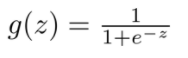
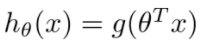
Decision boundary: find sigmoid function for multivariable linear regression equation,

Linear regression predicts in the whole real number domain with the same sensitivity, while the classification range needs to be [0,1]. Logistic regression is a one-step sigmoid nonlinear mapping based on linear regression. That is, a regression model that reduces the prediction range and limits the prediction value to [0,1]. Therefore, the linear regression model is sensitive to outliers, while the logical regression weakens the influence of points far away from the separation plane through nonlinear transformation, and its robustness is better than that of linear regression.

1.2 cost function

The cost function is a function that maps the value of a random event or its related random variables to a non negative real number to represent the "risk" or "loss" of the random event. It is used to evaluate the degree that the predicted value of the model is different from the real value. Generally, the smaller the cost function, the better the performance of the model.

linear regression

• Univariate linear regression:
  

• Multivariate linear regression:
  
  Among them,

• m: Number of training samples;

• h θ (x) : use parameters θ And the predicted y value of X;

• y: The y value in the original training sample, that is, the standard answer;

• Superscript (i): the ith sample.

logistic regression
For linear regression, J obtained by MSE is used( θ) It is a convex function, but for logistic regression, due to sigmoid nonlinear mapping, it is easy to fall into the problem of local optimization. Therefore, consider sigmoid as log to obtain J( θ).


J( θ) yes θ Find the second derivative and get that the second derivative is greater than 0, indicating J( θ) As a convex function, the global minimum can be found when the gradient descent method is used for optimization.

1.3 gradient descent method

The gradient descent algorithm is used to obtain the parameters that can minimize the cost function.

linear regression

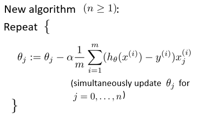
logistic regression

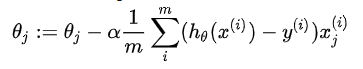
After the gradient descent algorithm, the formula forms of linear regression and logical regression seem to be the same, but in fact, they are completely different because the hypothetical functions are different.
Note: the normal equation can be used for linear regression to minimize the cost function θ， But logistic regression cannot use normal equation.

2 code implementation of linear regression

2.1 univariate linear regression

import numpy as np
import pandas as pd

# Read data
data = pd.read_csv(path, header=None, names=['x', 'y'])

# Cost function
def computeCost(X, y, theta):
    inner = np.power(((X * theta.T) - y), 2)
    return np.sum(inner) / (2 * len(X))

# Data processing and initialization
data.insert(0, 'Ones', 1) #Add a column to the training set so that the vectorized solution can be used to calculate the cost and gradient
cols = data.shape[1] #Gets the number of columns of the matrix
X = data.iloc[:,0:cols-1] #X is all rows, excluding the last column
y = data.iloc[:,cols-1:cols] #y is all rows, the last column

X = np.matrix(X.values)
y = np.matrix(y.values)
theta = np.matrix(np.array([0,0]))

computeCost(X, y, theta)

# Batch gradient descent algorithm
def gradientDescent(X, y, theta, alpha, iters):
    temp = np.matrix(np.zeros(theta.shape))
    parameters = int(theta.ravel().shape[1])
    cost = np.zeros(iters)
    
    for i in range(iters):
        error = (X * theta.T) - y
        
        for j in range(parameters):
            term = np.multiply(error, X[:,j])
            temp[0,j] = theta[0,j] - ((alpha / len(X)) * np.sum(term))
            
        theta = temp
        cost[i] = computeCost(X, y, theta)
        
    return theta, cost

alpha = 0.01 #Set learning rate α
iters = 2000 #Set the number of iterations

g, cost = gradientDescent(X, y, theta, alpha, iters) # Run the gradient descent algorithm to convert our parameters θ Suitable for training set
computeCost(X, y, g) #We use the fitted parameters to calculate the cost function of the training model

Visualization results

# Draw linear model
import matplotlib.pyplot as plt

x = np.linspace(data.x.min(), data.x.max(), 100)
f = g[0, 0] + (g[0, 1] * x)

fig, ax = plt.subplots(figsize=(12,8))
ax.plot(x, f, 'r', label='Prediction')
ax.scatter(data.x, data.y, label='Traning Data')
ax.legend(loc=2)
ax.set_xlabel('xxx')
ax.set_ylabel('xxx')
ax.set_title('xxx')
plt.show()

# Draw the relationship between the number of iterations and cost
fig, ax = plt.subplots(figsize=(12,8))
ax.plot(np.arange(iters), cost, 'r')
ax.set_xlabel('Iterations')
ax.set_ylabel('Cost')
ax.set_title('Error vs. Training Epoch')
plt.show()

2.2 multivariate linear regression

import pandas as pd

data = pd.read_csv(path, header=None, names=['x1', 'x2', 'y'])

# feature normalization 
data = (data - data.mean()) / data.std()

# Add ones to the first column
data.insert(0, 'Ones', 1)

cols = data.shape[1]
X = data.iloc[:,0:cols-1]
y = data.iloc[:,cols-1]

X = np.matrix(X.values)
y = np.matrix(y.values)
theta = np.matrix(np.array([0,0,0]))

# Call gradient descent algorithm
g, cost = gradientDescent(X, y, theta, alpha, iters)

computeCost(X, y, g2)

In addition to calling gradient descent algorithm, theta can also be obtained by using normal equation.

# Normal equation
def normalEqn(X, y):
    theta = np.linalg.inv(X.T@X)@X.T@y #X.T@X Equivalent to X.T.dot(X)
    return theta

Comparison between gradient descent and normal equation

• Gradient descent: need to choose learning rate α， It needs multiple iterations. When the number of features n is large, it can also be better applicable to various types of models
• Normal equation: no need to choose learning rate α， It can be calculated at one time, but it needs to be calculated ( X T X ) − 1 {{\left( {{X}^{T}}X \right)}^{-1}} (XTX)−1. If the number of features n is large, the operation cost is large, because the calculation time complexity of matrix inverse is O ( n 3 ) O(n3) O(n3), usually when n n When n is less than 10000, it is acceptable. It is only suitable for linear model, not suitable for other models such as logistic regression model

2.3 sklearn

from sklearn import linear_model

model = linear_model.LinearRegression()
model.fit(X, y)

x = np.array(X[:, 1].A1)
f = model.predict(X).flatten()


fig, ax = plt.subplots(figsize=(12,8))
ax.plot( x, f, 'r', label='Prediction')
ax.scatter(data.x, data.y, label='Traning Data')
ax.legend(loc=2)
ax.set_xlabel('x')
ax.set_ylabel('y')
ax.set_title('xxx')
plt.show()

Least squares linear regression: sklearn linear_ model. LinearRegression(fit_intercept=True, normalize=False,copy_X=True, n_jobs=1)

Description of main parameters

parameter	explain
fit_intercept	Boolean, the default is True. If the parameter value is True, it means that the training model needs to calculate intercept; If the parameter is False, it means that the intercept item does not need to be added to the model
normalize	Boolean, default to False, if fit_ When the intercept parameter is set to False, the normalize parameter does not need to be set; If normalize is set to True, the input sample data will be (X-X mean) / | X|; If normalize=False is set, sklearn can be used before training the model preprocessing. Standardize with standardscaler
copy_X	Boolean, the default is True, otherwise X will be overwritten
n_jobs	int, the default is 1, which indicates the number of jobs used for calculation. If - 1, it means calling all CPUs

attribute

• coef_: Regression coefficient (slope)

regr = linear_model.LinearRegression()
regr.fit(X,y)
regr.coef_

• intercept_: Intercept term

regr = linear_model.LinearRegression()
regr.fit(X,y)
regr.intercept_

Main methods

• fit(X, y, sample_weight=None), X and y are passed in as a matrix_ Weight is the weight of each test data, which is also passed in the form of matrix
• predict(X), a prediction method, is used to return the predicted value
• score(X, y, sample_weight=None), the scoring function will return a score less than 1, which may be less than 0
• get_params(deep=True) returns the setting value of the regressor

3 code implementation of logistic regression

3.1 logistic regression

import numpy as np
import pandas as pd
import matplotlib.pyplot as plt

data = pd.read_csv(path, header=None, names=['x1', 'x2', 'y'])

positive = data[data['y'].isin([1])]
negative = data[data['y'].isin([0])]

# Create a scatter plot of two "positive and negative" scores and use color coding to visualize them
fig, ax = plt.subplots(figsize=(12,8))
ax.scatter(positive['x1'], positive['x2'], s=50, c='b', marker='o', label='Yes')
ax.scatter(negative['x1'], negative['x2'], s=50, c='r', marker='x', label='No')
ax.legend()
ax.set_xlabel('x1 Score')
ax.set_ylabel('x2 Score')
plt.show()

# Define sigmoid function
def sigmoid(z):
    return 1 / (1 + np.exp(-z))

# Cost function definition
def cost(theta, X, y):
    theta = np.matrix(theta)
    X = np.matrix(X)
    y = np.matrix(y)
    first = np.multiply(-y, np.log(sigmoid(X * theta.T)))
    second = np.multiply((1 - y), np.log(1 - sigmoid(X * theta.T)))
    return np.sum(first - second) / (len(X))

# Data processing and initialization
data.insert(0, 'Ones', 1) #Insert ones
cols = data.shape[1] #Get the number of columns
X = data.iloc[:,0:cols-1]
y = data.iloc[:,cols-1:cols]

X = np.array(X.values)
y = np.array(y.values)
theta = np.zeros(3)

cost(theta, X, y)

# Gradient descent algorithm
def gradient(theta, X, y):
    theta = np.matrix(theta)
    X = np.matrix(X)
    y = np.matrix(y)
    
    parameters = int(theta.ravel().shape[1])
    grad = np.zeros(parameters)
    
    error = sigmoid(X * theta.T) - y
    
    for i in range(parameters):
        term = np.multiply(error, X[:,i])
        grad[i] = np.sum(term) / len(X)
    
    return grad

gradient(theta, X, y) #View the data and the results of the gradient descent method with an initial parameter of 0

# Using SciPy's truncated newton (TNC) to find the optimal parameters
import scipy.optimize as opt
result = opt.fmin_tnc(func=cost, x0=theta, fprime=gradient, args=(X, y))
cost(result[0], X, y)

# The obtained parameter theta is used to predict the output of data set X, and this function is used to score the training accuracy of the classifier.
def predict(theta, X):
    probability = sigmoid(X * theta.T)
    return [1 if x >= 0.5 else 0 for x in probability]

theta_min = np.matrix(result[0])
predictions = predict(theta_min, X)
correct = [1 if ((a == 1 and b == 1) or (a == 0 and b == 0)) else 0 for (a, b) in zip(predictions, y)]
accuracy = (sum(map(int, correct)) % len(correct))
print ('accuracy = {0}%'.format(accuracy))

If the original data has no obvious linear decision boundary, one method is to use the original feature polynomial to obtain the feature, and use the linear technology such as logistic regression for the feature.

degree = 5
x1 = data['Test 1']
x2 = data['Test 2']

data.insert(3, 'Ones', 1)

for i in range(1, degree):
    for j in range(0, i):
        data['F' + str(i) + str(j)] = np.power(x1, i-j) * np.power(x2, j)

data.drop('Test 1', axis=1, inplace=True)
data.drop('Test 2', axis=1, inplace=True)

# Regularization cost function
def costReg(theta, X, y, learningRate):
    theta = np.matrix(theta)
    X = np.matrix(X)
    y = np.matrix(y)
    first = np.multiply(-y, np.log(sigmoid(X * theta.T)))
    second = np.multiply((1 - y), np.log(1 - sigmoid(X * theta.T)))
    reg = (learningRate / (2 * len(X))) * np.sum(np.power(theta[:,1:theta.shape[1]], 2))
    return np.sum(first - second) / len(X) + reg

def gradientReg(theta, X, y, learningRate):
    theta = np.matrix(theta)
    X = np.matrix(X)
    y = np.matrix(y)
    
    parameters = int(theta.ravel().shape[1])
    grad = np.zeros(parameters)
    
    error = sigmoid(X * theta.T) - y
    
    for i in range(parameters):
        term = np.multiply(error, X[:,i])
        
        if (i == 0):
            grad[i] = np.sum(term) / len(X)
        else:
            grad[i] = (np.sum(term) / len(X)) + ((learningRate / len(X)) * theta[:,i])
    
    return grad

# Data initialization, X, y
cols = data.shape[1]
X = data.iloc[:,1:cols]
y = data.iloc[:,0:1]

X = np.array(X.values)
y = np.array(y.values)
theta = np.zeros(11)

learningRate = 1 # Initialization learning rate
costReg(theta, X, y, learningRate) #cost
gradientReg(theta, X, y, learningRate) #Get parameters

result = opt.fmin_tnc(func=costReg, x0=theta, fprime=gradientReg, args=(X, y, learningRate))
theta_min = np.matrix(result[0])
predictions = predict(theta_min, X)
correct = [1 if ((a == 1 and b == 1) or (a == 0 and b == 0)) else 0 for (a, b) in zip(predictions, y)]
accuracy = (sum(map(int, correct)) % len(correct))
print ('accuracy = {0}%'.format(accuracy))

3.2 sklearn

from sklearn import linear_model #Call the linear regression package of sklearn
model = linear_model.LogisticRegression(penalty='l2', C=1.0)
model.fit(X, y.ravel())

model.score(X, y)

reference material

logistic regression (derivation attached)
Linear regression and logistic regression
On machine learning: linear regression & logical regression
The code part mainly quotes the data of Dr. Huang haiguang