catalogue

• 1, Basic theory of multiple linear regression
• 2, Case analysis
• 3, Data preprocessing
• • 1. Error data cleaning
  • 2. Non numerical data conversion
• 4, Regression using Excel
• • 1. Regression realization
  • 2. Regression analysis
• 5, Regression using code
• • 1. Data preprocessing
  • 2. Use Statsmodels to establish multiple linear regression model
  • 3. Use Sklearn library to establish multiple linear regression model
  • 4. Model optimization
• 6, Summary
• 7, Reference

1, Basic theory of multiple linear regression

When studying practical problems, the change of dependent variables is often affected by several important factors. At this time, it is necessary to use two or more influencing factors as independent variables to explain the change of dependent variables, which is multiple regression. When there is a linear relationship between multiple independent variables and dependent variables, the regression analysis is multivariate regression. The mathematical model of linear regression is:
f ( x i ) = ω T x i + b f(\pmb x_i)=\pmb \omega^T \pmb x_i + b f(xxxi​)=ωωωTxxxi​+b

When sample X in dataset D I \ PMB x_ I XXXI is described by multiple attributes, which is called "multiple linear regression"

2, Case analysis

The trend of market house price is affected by many factors. Through the analysis of many factors affecting market house price, it is helpful to make a more accurate evaluation of the trend of house price in the future.
  through the linear regression analysis of the sold house price data in a certain area for a certain period of time, explore the main factors affecting the house price, analyze the influence degree of these factors, and use the data obtained from the analysis to predict the trend and trend of house price in the future.
  this paper explores the relationship between neighborhood, house area, bedrooms, bathrooms, house style and house price.

3, Data preprocessing

1. Error data cleaning

In the original data, it is found that there are suspected wrong data such as no bedroom, no bathroom or unreasonable house area. Therefore, the data will be properly cleaned first.

1. Select header and enable filtering

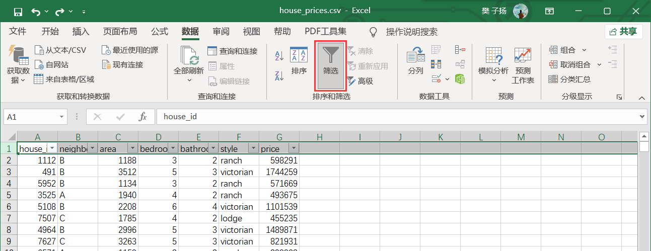
2. Select filter criteria and click OK (select data with bedrooms greater than 0 here)

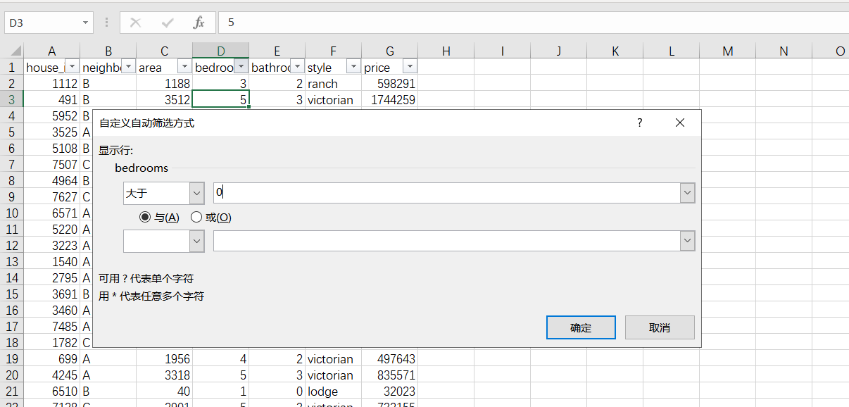
At this point, you can see that the data with bedrooms equal to 0 has been cleaned out.

Similarly, the data with bathrooms equal to 0 is cleaned out.

Then, the data with area less than 200 is cleaned.

Cleaning is complete.

2. Non numerical data conversion

In the original data, neighborhood and style are non numeric data. It needs to be converted into numerical data before regression analysis can be carried out.
  for neighborhood, replace A, B and C of the original data with 1, 2 and 3.
  for style, replace the ranch, victorian and lodge of the original data with 100, 200 and 300.

The replacement was successful and regression analysis can now be performed.

4, Regression using Excel

1. Regression realization

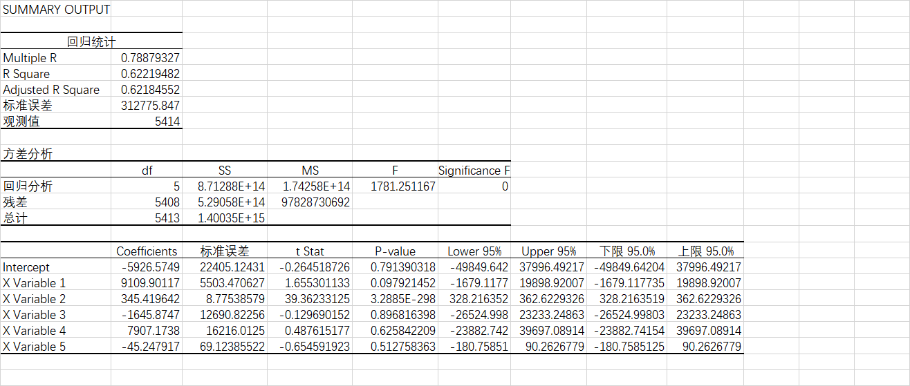
Take house price as dependent variable and other variables in the table as independent variables, and use Excel to conduct regression analysis on the data in the table.

2. Regression analysis

Regression statistical sub table analysis

Multiple R: correlation coefficient r, which is used to measure the correlation degree between independent variables x and y. The r = 0.788 obtained by regression analysis of this data set indicates that the relationship between x and Y is highly correlated.
R Square: determination coefficient R 2 R^2 R2
R 2 = 1 − ∑ i = 1 n ( y i − y ^ i ) 2 ∑ i = 1 n ( y i − y ˉ ) 2 R^2 = 1 - \frac{\sum_{i=1}^{n} (y_i - \hat{y}_i)2}{\sum_{i=1}{n} (y_i - \bar{y})^2} R2=1−∑i=1n​(yi​−yˉ​)2∑i=1n​(yi​−y^​i​)2​
   reflect the proportion that all variations of dependent variables can be explained by independent variables through regression relationship. It can be commonly understood as using the mean value as the error benchmark to see whether the prediction error is greater than or less than the mean value benchmark error. The R2 R ^ 2 R2 obtained from the regression analysis of this data set = 0.622, indicating that the independent variable can explain 62.2% of the dependent variable

Sub table III Analysis

independent variable	meaning	Coefficients
X Variable 1	Neighborhood	9109.90116615722
X Variable 2	House area	345.419642269034
X Variable 3	bedrooms	-1645.8747033071
X Variable 4	bathrooms	7907.17380048446
X Variable 5	House style	-45.2479173151558

According to the Coefficients in Table 3, the regression equation can be estimated as follows:
y = 9109.9 x 1 + 345.41 x 2 − 1645.87 x 3 + 7907.17 x 4 − 45.24 x 5 − 5926.57 y = 9109.9x_1 + 345.41x_2 - 1645.87x_3 + 7907.17x_4 - 45.24x_5 - 5926.57 y=9109.9x1​+345.41x2​−1645.87x3​+7907.17x4​−45.24x5​−5926.57
  however, there may be large errors in the regression equation estimated by Coefficients. More important is the P-value value value. It can be found from the value of P-value in the table that the independent variable house area x 2 x_ The p value of 2 X2 is far less than the significance level of 0.05, so the house area is related to the house price. The P values of bedrooms and bathrooms are much greater than the significance level of 0.05, indicating that the correlation between bedrooms and bathrooms and house price is weak, or even there is no linear correlation.

5, Regression using code

1. Data preprocessing

1. First, view the basic information of the data

import pandas as pd
import numpy as np
import seaborn as sns
import matplotlib.pyplot as plt#Import data
df = pd.read_csv("house_prices.csv")
#Read basic information of data
df.info()

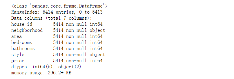
df.info(): returns some basic information of the table, mainly including the data type of each column of the dataset, whether it is null value and memory usage
RangeIndex: # rows, 5414
Data columns (total 7 columns): # number of columns, 7 columns
Non null: means non empty data
dtypes: int64(5), object(2): data type

1. Judgment and processing of redundant data

# Judge whether there are repeated observations in the data
df.duplicated().any()

If there are no duplicate data rows, it corresponds to False; otherwise, it corresponds to True.
False is returned here, indicating that there is no duplicate data in the data.

If there is duplicate data, use drop_ The duplicates() function deletes duplicate data

1. Missing value identification and processing

# Judge whether there are missing values in each variable
df.isnull().any(axis = 0)
# Number of missing values in each variable
df.isnull().sum(axis = 0)
# Proportion of missing values in each variable
df.isnull().sum(axis = 0)/df.shape[0]

No missing values were found in the data

1. Data outlier identification and processing

# Outlier handling
# ================Outlier test function: two methods of IQR & Z score=========================
def outlier_test(data, column, method=None, z=2):
    """ Based on a column, the upper and lower truncation point method is used to detect outliers(Indexes) """
    """ 
    full_data: Complete data
    column: full_data Specified column in, format 'x' Quoted
    return Optional; outlier: Outlier data frame 
    upper: Upper truncation point;  lower: Lower truncation point
    method: Method of checking outliers (optional), default None Is the upper and lower cut-off point method),
            choose Z Method, Z The default is 2
    """
    # ==================Upper and lower cut-off point method to test outliers==============================
    if method == None:
        print(f'with {column} Based on the column, the upper and lower cut-off point method is used(iqr) Detect outliers...')
        print('=' * 70)
        # Quartile; There will be exceptions when calling the function here
        column_iqr = np.quantile(data[column], 0.75) - np.quantile(data[column], 0.25)
        # 1, 3 quantiles
        (q1, q3) = np.quantile(data[column], 0.25), np.quantile(data[column], 0.75)
        # Calculate upper and lower cutoff points
        upper, lower = (q3 + 1.5 * column_iqr), (q1 - 1.5 * column_iqr)
        # Detect outliers
        outlier = data[(data[column] <= lower) | (data[column] >= upper)]
        print(f'First quantile: {q1}, Third quantile:{q3}, Interquartile range:{column_iqr}')
        print(f"Upper cutoff point:{upper}, Lower cutoff point:{lower}")
        return outlier, upper, lower
    # =====================Z-score test outliers==========================
    if method == 'z':
        """ Based on a column, the incoming data is the same as the data you want to segment z Score point, return the outlier index and the data frame """
        """ 
        params
        data: Complete data
        column: Specified detection column
        z: Z Quantile, The default is 2, according to z fraction-According to the normal curve table, take 2 at the left and right ends%，
           According to you z Positive and negative setting of scores. It can also be changed arbitrarily to know the data set of any top percentage
        """
        print(f'with {column} List as basis, use Z Fractional method, z Quantile extraction {z} To detect outliers...')
        print('=' * 70)
        # Calculate the numerical points of the two Z fractions
        mean, std = np.mean(data[column]), np.std(data[column])
        upper, lower = (mean + z * std), (mean - z * std)
        print(f"take {z} individual Z Score: greater than {upper} Or less than {lower} Is considered an outlier.")
        print('=' * 70)
        # Detect outliers
        outlier = data[(data[column] <= lower) | (data[column] >= upper)]
        return outlier, upper, lower

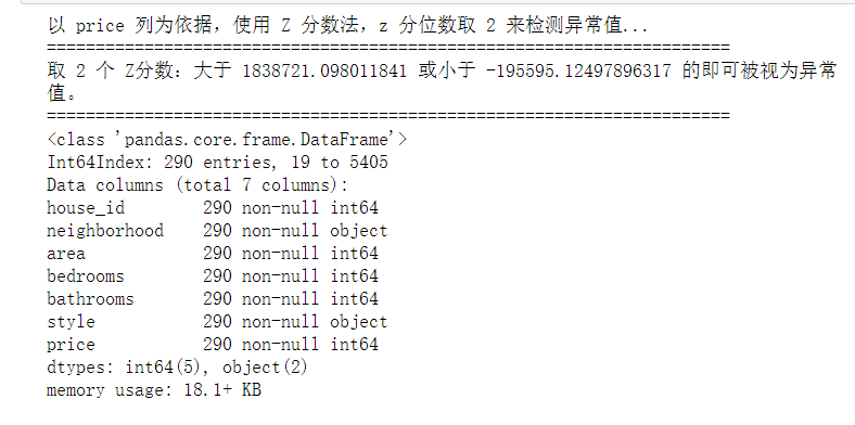
Perform anomaly detection‘

#Outlier detection of data
outlier, upper, lower = outlier_test(data=df, column='price', method='z')

outlier.info();
outlier.sample(5)

Discard outliers

# Simply discard it here
df.drop(index=outlier.index, inplace=True)

1. Statistical non numerical variable

# Category variables, also known as nominal variables
nominal_vars = ['neighborhood', 'style']

for each in nominal_vars:
    print(each, ':')
    print(df[each].agg(['value_counts']).T)
    # Direct value_counts().T cannot achieve the following effect
    ## You must get agg, and the brackets [] inside can't be less
    print('='*35)
    # It is found that the number of each category is also OK, so as to prepare for the following analysis of variance

Draw a thermodynamic diagram

# Thermodynamic diagram 
def heatmap(data, method='pearson', camp='RdYlGn', figsize=(10 ,8)):
    """
    data: Whole data
    method: Default to pearson coefficient
    camp: The default is: RdYlGn-Red, yellow and blue; YlGnBu-Yellow green blue; Blues/Greens It's also a good choice
    figsize: The default is 10, 8
    """
    ##    Eliminate color blocks with diagonal color duplication
    #     mask = np.zeros_like(df2.corr())
    #     mask[np.tril_indices_from(mask)] = True
    plt.figure(figsize=figsize, dpi= 80)
    sns.heatmap(data.corr(method=method), \
                xticklabels=data.corr(method=method).columns, \
                yticklabels=data.corr(method=method).columns, cmap=camp, \
                center=0, annot=True)
    # To achieve the effect of leaving only half of the diagonal, the parameters in brackets can be added with mask=mask

heatmap(data=df, figsize=(6,5))

   it can be seen from the thermodynamic diagram that the relationship between variables such as area, bedrooms and bathrooms and house price is still relatively strong, so it is worth putting into the model, but the relationship between classified variables style and neighborhood and price is unknown.

1. variance analysis

In the exploration just now, we found that the categories of style and neighborhood are three categories. If there are only two categories, we can conduct chi square test, so here we use analysis of variance.

## Using analysis of variance in regression model
## Only statsmodels have ANOVA libraries
## The analysis of variance results were extracted from the linear regression results
import statsmodels.api as sm
from statsmodels.formula.api import ols # ols is a statistical database for establishing linear regression model
from statsmodels.stats.anova import anova_lm

Sample size and confidence level α_ Attention points of level (confidence level) α Selection experience)
Sample size α- level
≤ 100 10%
100 ＜ n ≤ 500 5%
500 ＜ n ≤ 1000 1%
n ＞ one thousandth of 2000
The sample size is too large, α- level is meaningless.
When the data volume is large, the p value is useless, and the sample size usually does not exceed 5000,
In order to prove that the relationship between the two variables is stable, the sample size should be well controlled.

# Select 600 samples randomly from the data set. If you want stratified sampling, please refer to the article:
df = df.copy().sample(600)

# C means to tell python that this is a classified variable, otherwise Python will use it as a continuous variable
## Here, analysis of variance is directly used to test all classified variables
## The following lines of code are the standard gestures for analysis of variance using the statistical library
lm = ols('price ~ C(neighborhood) + C(style)', data=df).fit()
anova_lm(lm)

# The Residual line indicates the within group that cannot be explained by the model, and the others are between groups that can be explained
# df: degree of freedom (n-1) - the number of categories in the classification variable minus 1
# sum_sq: sum of total squares (SSM), sum of residual lines_ eq: SSE
# mean_ SQ: MSM, mean of residual line_ sq: mse
# F: F statistics, just check the chi square distribution table
# Pr (> F): P value

Refresh several times and find that they are very significant, so these two variables are also worth putting into the model

2. Use Statsmodels to establish multiple linear regression model

Here, the least square method is directly used to establish the linear regression model

from statsmodels.formula.api import ols
#Establishment of linear regression model by least square method
lm = ols('price ~ area + bedrooms + bathrooms', data=df).fit()
lm.summary()

The fitting effect of the model is not ideal, R2 = 0.54, R ^ 2 = 0.54, R2 = 0.54, and the model needs to be further optimized.

3. Use Sklearn library to establish multiple linear regression model

• Import related libraries

#Import related libraries
import pandas as pd
import numpy as np
from sklearn.model_selection import train_test_split #Cross validation is referenced here
from sklearn.linear_model import LinearRegression  #linear regression
from sklearn.linear_model import Lasso, Ridge, LinearRegression as LR
from sklearn.metrics import r2_score, explained_variance_score as EVS, mean_squared_error as MSE
from sklearn.model_selection import train_test_split, cross_val_score
from pandas.core.accessor import register_dataframe_accessor

• read in data

#read in data
data=pd.read_csv('house_prices.csv')
x = data[['neighborhood','area','bedrooms','bathrooms','style']]# Characteristic data, independent variable
y= data['price']# Tag value, dependent variable

• Data set partition

#It is divided into training set and test set in the proportion of 8:2
x_train, x_test, y_train, y_test = train_test_split(
    x, y, test_size=0.2, random_state=1)

• Model training and solution

reg = LR().fit(x_train, y_train)  # Training model
yhat = reg.predict(x_test)  # Label prediction based on test set x
print("r2 = ",r2_score(y_test,yhat))#Decision coefficient R^2

• Save file

f = open("multiple linear regression .txt", 'w+', encoding='utf8')
f.write("The parameters are:" + str(reg.coef_)+"\t\n")  # The coefficients of each feature are obtained
f.write("Intercept is:" + str(reg.intercept_)+"\t\n")  # Get the intercept, constant c
f.write("The mean square deviation is:" + str(MSE(y_test, yhat))+"\t\n")  # Mean square deviation (absolute value)
f.write('The ratio of the average error to the average of the real value of the sample is:'+str(np.sqrt(MSE(y_test, yhat)) /y_test.mean())+"\t\n")  # The ratio of the average error to the average of the real value of the sample
f.write("Determination coefficient R^2 Is:"+str(r2_score(y_test,yhat))+"\t\n")
#Print ("the mean value of R ^ 2 is:", r2_score(y_test,yhat))
f.write(("The interpretable variance is:"+str(cross_val_score(reg, x, y, cv=5, scoring="explained_variance")) ))
f.close()

The accuracy of linear regression model based on Sklearn is higher than that based on Statsmodels.

4. Model optimization

Due to the low accuracy of the model, the accuracy of the model is improved by adding dummy variables and using variance expansion factor to detect multicollinearity.

# Set dummy variable
# Take the nominal variable neighborhood as an example
nominal_data = df['neighborhood']

# Set dummy variable
dummies = pd.get_dummies(nominal_data)
dummies.sample()  # pandas will automatically name it for you

# One dummy variable generated by each nominal variable needs to be discarded. Here, take discarding C as an example
dummies.drop(columns=['C'], inplace=True)
dummies.sample()

Splice the results with the original data set

# Splice the results with the original data set
results = pd.concat(objs=[df, dummies], axis='columns')  # Merge by column
results.sample(3)
# You can try to handle the nominal variable style by yourself

Modeling again

lm = ols('price ~ area + bedrooms + bathrooms + A + B', data=results).fit()
lm.summary()

At this time, R2 = 0.92, R ^ 2 = 0.92, R2 = 0.92, because the model accuracy is ideal.

6, Summary

In fact, multiple linear regression is the generalization of simple linear regression, in which the input x changes from a single feature to a vector containing n features. In multiple linear regression, it is only considered that there is a simple weighted summation relationship between each feature and the predicted value. This assumption is often far fetched, resulting in unsatisfactory accuracy, but it does work well in some applications.

Compared with Excel for data cleaning and processing, Pandas library provides better data cleaning and processing ability. At the same time, Python can more flexibly optimize the model and improve the accuracy.

By using statistical analysis, Statsmodels library and linear regression in Sklearn_ The model library carries out regression analysis on the same problem. The two methods have their own advantages and disadvantages. When using the statistical analysis Statsmodels library, it can be found that the regression analysis can be carried out directly without converting non numerical data, but at the same time, the accuracy of the model is greatly reduced. While using Excel and linear_model, non numerical data must be converted to numerical data.

7, Reference

House price forecast based on multiple linear regression

Detailed explanation of multiple linear regression analysis theory of machine learning algorithm (8)

Machine learning theory (3) multiple linear regression

This article is transferred from https://blog.csdn.net/YangMax1/article/details/120812509 , in case of infringement, please contact to delete.