Implementation of nonlinear support vector machine

Suppose that the nonlinear problem we face is the following two classification problem:

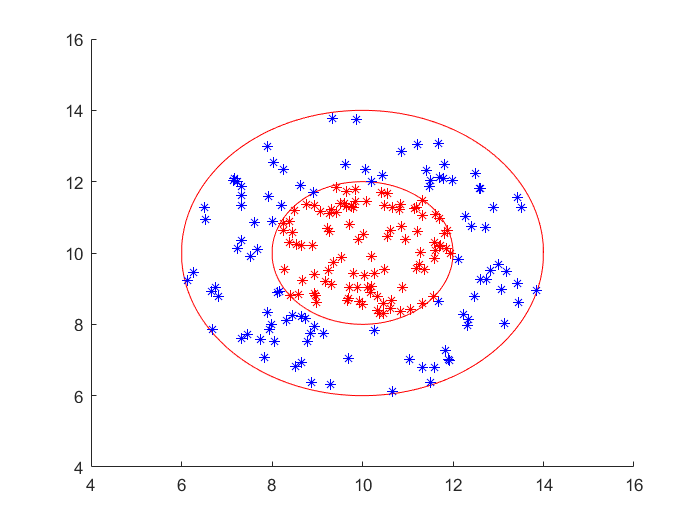
   it requires us to find a suitable curve that can correctly distinguish red and blue sample points. There is no doubt that linear support vector machine can not solve this kind of problem. We can solve the problem with the help of nonlinear support vector machine. Then the following core problem is to find the appropriate kernel function. When we don't know what kernel function is appropriate, It is a good idea to give priority to Gaussian kernel function. Namely:
K ( x , z ) = e x p ( − ∣ ∣ x − z ∣ ∣ 2 2 σ 2 ) K(x,z)=exp(-\frac{||x-z||^2}{2\sigma^2 }) K(x,z)=exp(−2σ2∣∣x−z∣∣2​)
Then the following mathematical model can be programmed:

Dual problem of nonlinear support vector machine
min ⁡ α       1 2 ∑ i = 1 N ∑ j = 1 N α i α j y i y j K ( x i , x j ) − ∑ i = 1 N α i s . t .       ∑ i = 1 N α i y i = 0 0 ≤ α i ≤ C       i = 1 , 2 , ⋯   , N \min\limits_{\alpha}\,\,\,\,\,\frac{1}{2}\sum\limits_{i=1}^N{\sum\limits_{j=1}^N{\alpha_i\alpha_jy_iy_jK(x_i,x_j) }}-\sum\limits_{i=1}^N{\alpha_i}\\ s.t.\,\,\,\,\,\sum\limits_{i=1}^N\alpha_i y_i=0\\ 0\le\alpha_i\le C\,\,\,\,\,i=1,2,\cdots,N αmin​21​i=1∑N​j=1∑N​αi​αj​yi​yj​K(xi​,xj​)−i=1∑N​αi​s.t.i=1∑N​αi​yi​=00≤αi​≤Ci=1,2,⋯,N

   in fact, compared with linear support vector machine, the biggest difference is that the inner product of the original feature vector is replaced with the form of kernel function, so the calculation method is only changed in the programming implementation, and finally there is no need to calculate w w The value of w only needs to construct the decision function. The code is as follows:
Training code:

%% Nonlinear SVM Test two
%% Empty variable
clc;
clear;

%% Call the drawing function and return the data to be drawn
data = plot_Circle(10,10,4,2,100);
X = data(:,1:2);
y = data(:,3);

%% Using kernel function to train existing data
cig = 1;
C = 10;
% Classification using kernel technique is still a quadratic programming solution
% Constructing quadratic coefficient matrix H
H = [];
for i =1:length(X)
    for j = 1:length(X)
        H(i,j) = exp(-(norm(X(i,:) - X(j,:)))/(2*cig^2))*y(i)*y(j);
    end
end
% exp(-(norm(X(i,:) - X(j,:)))/(2*cig^2))
% Construct first-order term coefficient f
f = zeros(length(X),1)-1;
A = [];b = []; % Inequality constraint
Aeq = y';beq = 0; % Equality constraint
ub = ones(length(X),1).*C;lb = zeros(length(X),1); % Range of arguments
[x,fval] = quadprog(H,f,A,b,Aeq,beq,lb,ub);
% x Represents the solution of the argument, and x Function value at
% Will be very small x Direct assignment to 0
x(x < 1e-5) = 0;
% solve b Value of
[a,~] = find(x~=0); % Find a solution b Value of
B = 0;
for i =1:length(X)
    B = B + x(i)*y(i)*exp(-(norm(X(i,:) - X(a(1),:)))/(2*cig^2));
end
b = y(a(1)) - B;

Test code:

%% Test on test set
random = unifrnd(6,14,2000,2); % Generate data to be predicted
yuce = zeros(length(random),1);
for i =1:length(random)
    F = 0;
    for j =1:length(x)
        F = F + x(j)*y(j)*exp(-(norm(X(j,:) - random(i,:)))/(2*cig^2));
    end
    f = F + b;
    if f > 0
        yuce(i) = 1;
    elseif f < 0
        yuce(i) = -1;
    end
end
yuce_1 = [];
yuce_2 = [];
for i =1:length(yuce)
    if yuce(i) == 1
        yuce_1 = [yuce_1;random(i,:)];
    else
        yuce_2 = [yuce_2;random(i,:)];
    end
end
% Plot the error on the test set
figure(2)
scatter(yuce_1(:,1),yuce_1(:,2),'*');
hold on
scatter(yuce_2(:,1),yuce_2(:,2),'*');
xlim([4,16]);
ylim([4,16])

   I divide the whole part into two parts. The first is the training data, and then the prediction data. Since the learning process of nonlinear support vector machine is not explicit learning, we can't find the functional formula of hyperplane in the solution process, but when we use the test set for testing, the results on the two-dimensional plane can be visualized, When I was testing, I randomly generated 20000 points in the range, and then called the decision function to predict the results.

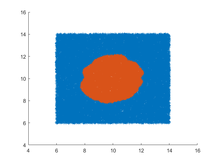
The visualization results also show that the learning algorithm is reliable, and the number of support vectors is found, α > 0 \alpha>0 α> There are 66 samples of 0, but there is no explicit equation of support vector machine.