1, Data set description
1. Data set
 https://www.kaggle.com/c/tabular-playground-series-feb-2022/data
For this challenge, you will predict bacterial species based on repeated lossy measurements of DNA fragments. The fragment with length of 10 is analyzed by Raman spectrum, which calculates the histogram of bases in the fragment.
Each row of data contains a histogram generated by repeated measurement samples, each row contains the output of all 286 histogram possibilities, and then the deviation spectrum (completely random) is subtracted from the result.
The data (training and testing) also contains simulated measurement errors (rate of change) of many samples, which makes the problem more challenging.
2. Preliminary observation
The target column is the target variable and is controlled by Streptoccus_ pyogenes,Salmonella_enterica,Enterococcus_hirae,Escherichia_coli,Campylobacter_jejuni,Streptococcus_pneumoniae,Staphylococcus_aureus,Escherichia_fergusonii,Bacteroides_fragilis,Klebsiella_pneumoniae and other 10 kinds of bacteria.
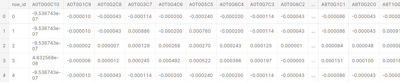
The training data set has 200000 rows and 288 columns, including 286 features, 1 target variable target and 1 row column_ id.
The test data set has 100000 rows and 287 columns, including 286 features, one of which is row_id.
There were no missing values in the training and test data sets.
2, Exploratory analysis
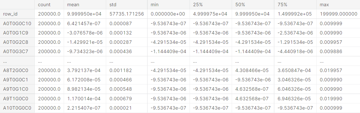
1. Data summary
df_train.describe().T
2. Data type
row_id is int64 bit, target is object, and other data is float64 bit.
df_train.info()
<class 'pandas.core.frame.DataFrame'>
RangeIndex: 200000 entries, 0 to 199999
Columns: 288 entries, row_id to target
dtypes: float64(286), int64(1), object(1)
memory usage: 439.5+ MB
3. Duplicate view of data
First remove row_id column
data = pd.read_csv('data/train.csv')
del data['row_id']
# Find duplicates
duplicates_train = data.duplicated().sum()
print('Duplicates in train data: {0}'.format(duplicates_train))

# To repeat
data.drop_duplicates(keep='first', inplace=True)
duplicates_train = data.duplicated().sum()

print('Train data shape:', data.shape)
print('Duplicates in train data: {0}'.format(duplicates_train))
It can be seen that there are duplicate data, and it is necessary to consider whether to remove it in the later processing.
Duplicates in train data: 76007
Train data shape: (123993, 287)
Duplicates in train data: 0
4. View data distribution
import plotly.graph_objects as go
fig = go.Figure()
fig.add_trace(go.Pie(values = target_class['count'],labels = target_class.index,hole = 0.6,
                     hoverinfo ='label+percent'))
fig.update_traces(textfont_size = 12, hoverinfo ='label+percent',textinfo='label',
                  showlegend = False,marker = dict(colors =["#201E1F","#FF4000","#FAAA8D","#FEEFDD","#50B2C0",
                                                            "#390099","#9e0059","#ff0054","#38B000","#ffbd00"]),
                  title = dict(text = 'Target Distribution'))
fig.show()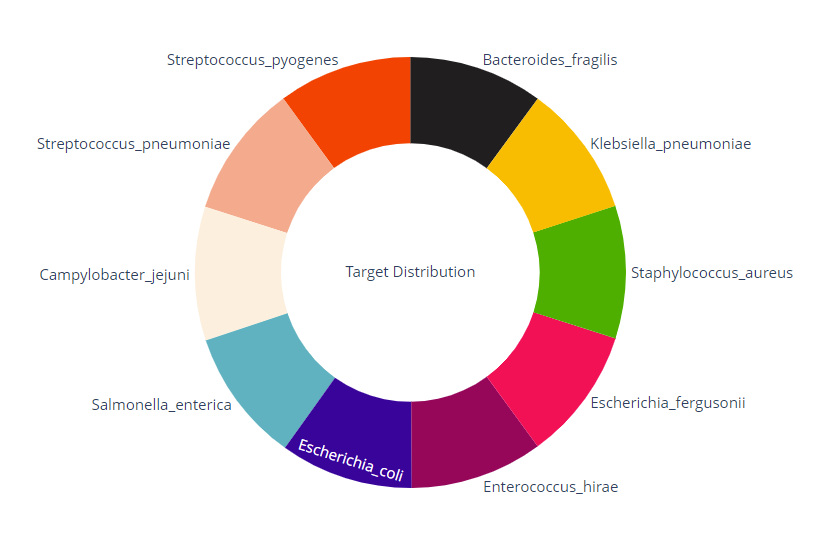
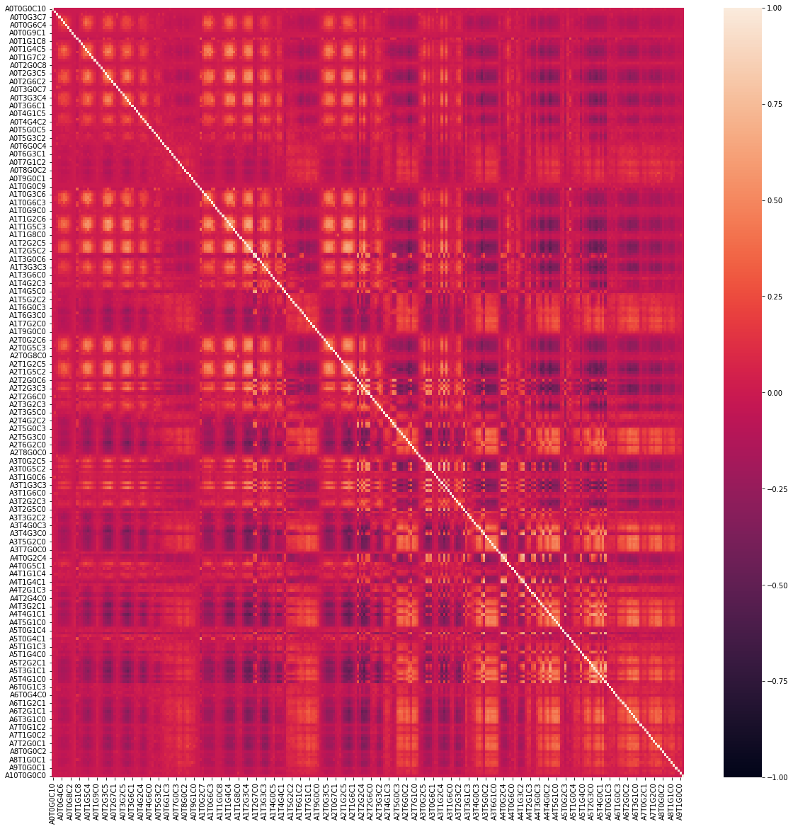
5. Correlation analysis
f, ax = plt.subplots(figsize=(20,20))
ax = sns.heatmap(df.corr(), vmin=-1, vmax=+1)
plt.show()
6. Characteristic distribution
rows, cols = 56, 5
f, axs = plt.subplots(nrows=rows, ncols=cols, figsize=(20, 200))
f.set_facecolor("#fff")
n_feat = 0
for row in tqdm(range(rows)):
    for col in range(cols):
        try:
            sns.kdeplot(x=NUM_FEATURES[n_feat], fill=True, alpha=1, linewidth=3,
                                        edgecolor="#264653", data=df, ax=axs[row, col], color='w')
            axs[row, col].patch.set_facecolor("#619b8a")
            axs[row, col].patch.set_alpha(0.8)
            axs[row, col].grid(color="#264653", alpha=1, axis="both")
        except IndexError: # hide last empty graphs
            axs[row, col].set_visible(False)
        n_feat += 1

f.show()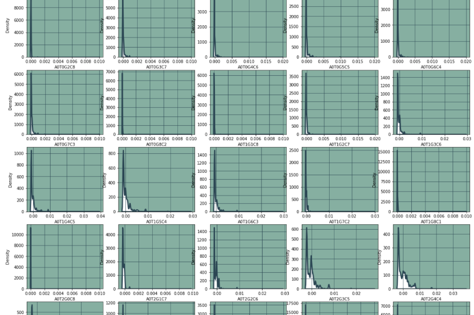
7. Numerical discreteness
Although the feature is a floating-point number, there are not 200000 unique values, but only about 100.
The last digits are always the same (from 1.00846558e-05 to 9.70846558e-05, they always end with 0846558).
This observation strongly suggests that these values are initially integers. Divide these integers by 1000000 and subtract a constant.
The paper given by kaggle describes this process and gives the formula of addition constant, which they call deviation. With this formula, we can convert floating-point numbers back to original integers:
 https://www.frontiersin.org/articles/10.3389/fmicb.2020.00257/full
def bias(w, x, y, z):
    return factorial(10) / (factorial(w) * factorial(x) * factorial(y) * factorial(z) * 4**10)

def bias_of(s):
    w = int(s[1:s.index('T')])
    x = int(s[s.index('T')+1:s.index('G')])
    y = int(s[s.index('G')+1:s.index('C')])
    z = int(s[s.index('C')+1:])
    return factorial(10) / (factorial(w) * factorial(x) * factorial(y) * factorial(z) * 4**10)

train_i = pd.DataFrame({col: ((train_df[col] + bias_of(col)) * 1000000).round().astype(int)
                        for col in elements})
test_i = pd.DataFrame({col: ((test_df[col] + bias_of(col)) * 1000000).round().astype(int)
                       for col in elements})
train_i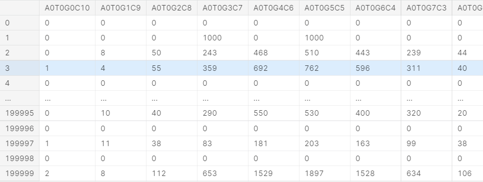
Calculate the maximum common divisor according to the above raw data,
# def gcd_of_all(df_i):
#     gcd = df_i[elements[0]]
#     for col in elements[1:]:
#         gcd = np.gcd(gcd, df_i[col])
#     return gcd

train_df['gcd'] = np.gcd.reduce(train_i[elements], axis=1)
test_df['gcd'] = np.gcd.reduce(test_i[elements], axis=1)
# train_df['gcd'] = train_i[elements].apply(np.gcd.reduce, axis=1) # slow
# test_df['gcd'] = test_i[elements].apply(np.gcd.reduce, axis=1)
# train_df['gcd'] = gcd_of_all(train_i)
# test_df['gcd'] = gcd_of_all(test_i)
np.unique(train_df['gcd'], return_counts=True), np.unique(test_df['gcd'], return_counts=True)
((array([    1,    10,  1000, 10000]), array([49969, 50002, 50058, 49971])),
 (array([    1,    10,  1000, 10000]), array([25208, 24951, 24930, 24911])))
We see four gcd values of the same frequency (1, 10, 1000 and 10000). Connecting this result with what they wrote in the paper, we understand this part of the experiment:
For each line, they extracted the bacterial DNA and cut it into decamers (DNA substrings with a length of 10). Then they put 1000000, 100000, 1000 or 100 decamers into their machine, which calculated how many times each of the 286 types from A0T0G0C10 to A10T0G0C0 appeared. This is what they call the spectrum (also known as a histogram with 286 bin). They standardized the spectrum by dividing all counts by the sum of the rows and subtracting the deviation.
Each bacterium has its own characteristic spectrum, and the competitive task is to predict the name of the bacterium from the spectrum of the sample. If the sample spectrum consists of one million decimal, we will accurately estimate the real frequency and predict the name easily; If the spectrum consists of only 100 decamers, we have little information and it will be difficult to predict (category overlap). We can see the influence of decamer number in the following four PCA diagrams:
for scale in np.sort(train_df['gcd'].unique()):
    # Compute the PCA
    pca = PCA(whiten=True, random_state=1)
    pca.fit(train_i[elements][train_df['gcd'] == scale])

    # Transform the data so that the components can be analyzed
    Xt_tr = pca.transform(train_i[elements][train_df['gcd'] == scale])
    Xt_te = pca.transform(test_i[elements][test_df['gcd'] == scale])

    # Plot a scattergram, projected to two PCA components, colored by classification target
    plt.figure(figsize=(6,6))
    plt.scatter(Xt_tr[:,0], Xt_tr[:,1], c=train_df.target_num[train_df['gcd'] == scale], cmap='tab10', s=1)
    plt.title(f"{1000000 // scale} decamers ({(train_df['gcd'] == scale).sum()} samples with gcd = {scale})")
    plt.show()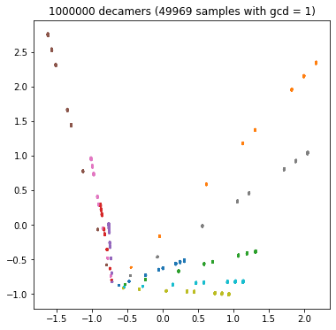
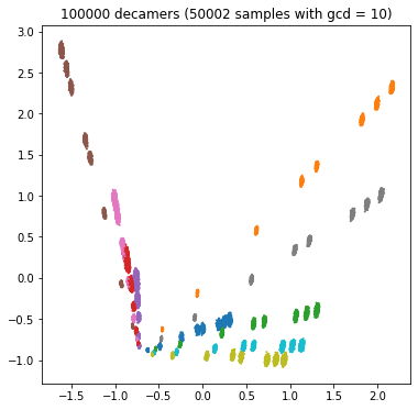
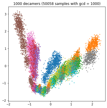
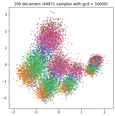
We might want to create four separate classifiers for the four GCD values. For GCD = 1, we expect high accuracy; For GCD = 10000, the accuracy will be lower.
If we only create one classifier, gcd can be used as an additional function.