logistic regression

summary

What is logistic regression

Although Logistic Regression is called regression, it is actually a classification model, which is often used in secondary classification. Logistic Regression is widely used because of its simplicity, parallelization and strong interpretability. Second classification (also known as logical classification) is a common classification method, which divides a batch of samples or data into two categories. For example, an examination can be divided into pass and fail according to the results, as shown in the following table:

This is logical classification, which maps continuous values into two categories.

Logic function

Logistic regression is a kind of generalized linear regression. Its principle is to use the linear model to calculate the output according to the input (the output value of the linear model is continuous), and convert the continuous value into two discrete values (0 or 1) under the action of the logical function. Its expression is as follows:

y = h(w_1x_1 + w_2x_2 + w_3x_3 + ... + w_nx_n + b)

Among them, the part in brackets is a linear model, and the calculation results are converted into binary under the action of function h(). The definition of function h() is:

h= \frac{1}{1+e^{-t}}

t=w^Tx+b

This function is called Sigmoid function (also known as logic function), which can map the value of (− ∞, + ∞) to (0,1). Its image is:

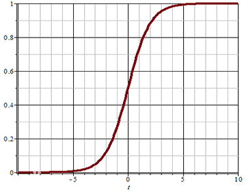
You can set a threshold (for example, 0.5). When the value of the function is greater than the threshold, the classification result is 1; When the function value is less than the threshold, the classification result is 0 This threshold can also be adjusted according to the actual situation

Classification of loss function

For the regression problem, the mean square deviation can be used as the loss function. For the classification problem, how to measure the difference between the predicted value and the real value? The classification problem adopts cross entropy as the loss function. When there are only two categories, the expression of cross entropy is:

E(y, \hat{y}) = -[y \ log(\hat{y}) + (1-y)log(1-\hat{y})]

Where y is the real value and hat{y} is the predicted value

• When y=1, the closer the predicted value \ hat{y} is to 1, the closer the log(\hat{y}) is to 0, and the smaller the loss function value is, the smaller the error is, and the more accurate the prediction is; When the prediction time \ hat{y} is close to 0, the log(\hat{y}) is close to negative infinity. The greater the error after adding the symbol, the more inaccurate it is;
• When y=0, the closer the predicted value \ hat{y} is to 0, the closer the log(1-\hat{y}) is to 0, and the smaller the loss function value is, the smaller the error is, and the more accurate the prediction is; When the predicted value \ hat{y} is close to 1, log(1-\hat{y}) is close to negative infinity. The greater the error after adding symbols, the more inaccurate it is

Logistic regression implementation

In sklearn, the relevant API s of logistic regression are as follows:

# Model creation
# solver parameter: the functional relationship of the exponent in the logical function (liblinear indicates linear relationship)
# Parameter C: the larger the regularization intensity, the smaller the fitting effect. Adjust this parameter to prevent over fitting
model = lm.LogisticRegression(solver='liblinear', C=1)

# train
model.fit(x, y) 

# forecast
pred_y = model.predict(x)

The following is the code implemented using the logical progression provided by the sklearn Library:

# Logical classifier example
import numpy as np
import sklearn.linear_model as lm
import matplotlib.pyplot as mp

x = np.array([[3, 1], [2, 5], [1, 8], [6, 4],
              [5, 2], [3, 5], [4, 7], [4, -1]])
y = np.array([0, 1, 1, 0, 0, 1, 1, 0])

# Create logical classifier object
model = lm.LogisticRegression()
model.fit(x, y)  # train

# forecast
test_x = np.array([[3, 9], [6, 1]])
test_y = model.predict(test_x)  # forecast
print(test_y)

# Calculate the boundaries of the displayed coordinates
left = x[:, 0].min() - 1
right = x[:, 0].max() + 1
buttom = x[:, 1].min() - 1
top = x[:, 1].max() + 1

# Generate gridded matrix
grid_x, grid_y = np.meshgrid(np.arange(left, right, 0.01),
                             np.arange(buttom, top, 0.01))

print("grid_x.shape:", grid_x.shape)
print("grid_y.shape:", grid_y.shape)

# Merge the x,y coordinates into two columns
mesh_x = np.column_stack((grid_x.ravel(), grid_y.ravel()))
print("mesh_x.shape:", mesh_x.shape)

# Predict according to the xy coordinates of each point and restore it to a two-dimensional shape
mesh_z = model.predict(mesh_x)
mesh_z = mesh_z.reshape(grid_x.shape)

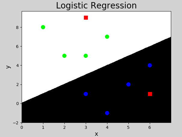
mp.figure('Logistic Regression', facecolor='lightgray')
mp.title('Logistic Regression', fontsize=20)
mp.xlabel('x', fontsize=14)
mp.ylabel('y', fontsize=14)
mp.tick_params(labelsize=10)
mp.pcolormesh(grid_x, grid_y, mesh_z, cmap='gray')
mp.scatter(x[:, 0],  # Sample x coordinate
           x[:, 1],  # Sample y coordinate
           c=y, cmap='brg', s=80)
mp.scatter(test_x[:, 0], test_x[:, 1], c="red", marker='s', s=80)
mp.show()

Execution result:

Supplement: L-BFGS algorithm

Multi classification implementation

Logistic regression produces two classification results, which can be realized by multiple binary classifiers (one multivariate classification problem is transformed into multiple binary classification problems) If there are the following sample data:

The following classifications were carried out for several times and the results were obtained:

The first time: it is divided into class A (value is 1) and non class A (value is 0)

The second time: it is divided into class B (value is 1) and non class B (value is 0)

The third time: it is divided into class C (value is 1) and non-C (value is 0)

......

and so on.

The example code of multiple classification using logical classifier is as follows:

# Multivariate classifier example
import numpy as np
import sklearn.linear_model as lm
import matplotlib.pyplot as mp

# input
x = np.array([[4, 7],
              [3.5, 8],
              [3.1, 6.2],
              [0.5, 1],
              [1, 2],
              [1.2, 1.9],
              [6, 2],
              [5.7, 1.5],
              [5.4, 2.2]])
# Output (multiple categories)
y = np.array([0, 0, 0, 1, 1, 1, 2, 2, 2])

# Create logical classifier object
model = lm.LogisticRegression(C=200) # Adjust the value to 1 to see the effect
model.fit(x, y)  # train

# Axis range
left = x[:, 0].min() - 1
right = x[:, 0].max() + 1
h = 0.005

buttom = x[:, 1].min() - 1
top = x[:, 1].max() + 1
v = 0.005

grid_x, grid_y = np.meshgrid(np.arange(left, right, h),
                             np.arange(buttom, top, v))

mesh_x = np.column_stack((grid_x.ravel(), grid_y.ravel()))
mesh_z = model.predict(mesh_x)
mesh_z = mesh_z.reshape(grid_x.shape)

# visualization
mp.figure('Logistic Classification', facecolor='lightgray')
mp.title('Logistic Classification', fontsize=20)
mp.xlabel('x', fontsize=14)
mp.ylabel('y', fontsize=14)
mp.tick_params(labelsize=10)
mp.pcolormesh(grid_x, grid_y, mesh_z, cmap='gray')
mp.scatter(x[:, 0], x[:, 1], c=y, cmap='brg', s=80)
mp.show()

Execution result:

summary

1) Logistic regression is a classification problem, which is used to realize two classification problems

2) Implementation method: using linear model calculation to generate classification under the action of logic function

3) Multi classification implementation: multi classification problems can be transformed into two classification problems

4) Purpose: widely used in various classification problems