Artificial intelligence course overview

What is artificial intelligence

Artificial Intelligence is a branch of computer science. It mainly studies how to simulate people's way of thinking and behavior with computers, so as to replace people in some fields

Discipline system of artificial intelligence

The following is the discipline system diagram of artificial intelligence:

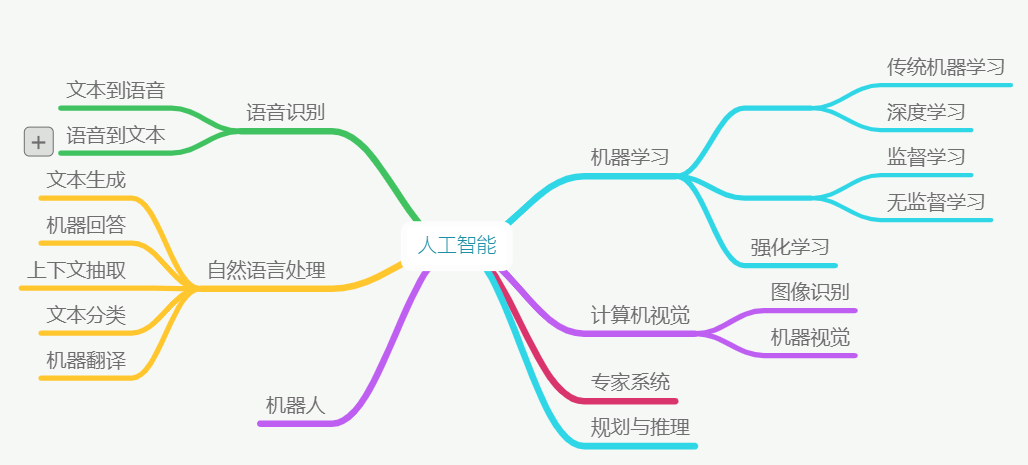
• Machine Learning: a sub discipline of artificial intelligence, which studies the basic algorithms, principles and ideas in the field of artificial intelligence. The research content of Machine Learning will be used in other sub disciplines
• Computer Vision: study the related technologies of computer processing, recognition and understanding of images and videos
• Natural Language Processing (NLP): Research on computer understanding of human natural language related technologies
• Language processing: study the related technologies of computer recognition, understanding and speech synthesis

The difference between artificial intelligence and traditional software

• Traditional software: execute people's instructions and ideas. Predecessors have had solutions before the implementation, which can not go beyond the scope of people's thoughts and understanding
• Artificial intelligence: try to break through the scope of people's thought and understanding, let the computer learn new abilities, and try to solve the problems of traditional software

Course introduction

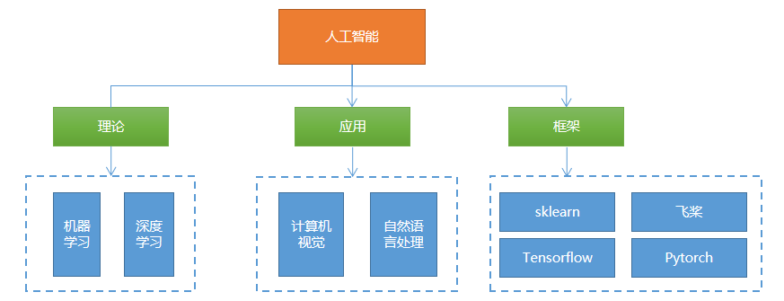
Course content

The course contents mainly include:

Course characteristics

• Many contents: including machine learning, deep learning, computer vision, NLP and common frameworks
• Difficulty: it is difficult to learn, to get started, to improve and to apply
• Need some mathematical knowledge: remember the conclusion, call API, analyze formula and deduce formula
• Need to learn repeatedly: the first round of understanding the main content, the second round of understanding the core concepts, the third round of familiarity with code writing, and the fourth round of in-depth understanding and application
• The more you learn, the deeper you get

learning method

• Understand first and understand again
• First easy then difficult, first listen then write, first coarse then fine
• Skip the difficult knowledge points and focus on the big and let go of the small
• Read more textbooks from different authors and listen to more explanations from different teachers

Basic concepts of machine learning

What is machine learning

Herbert, winner of Turing prize in 1975, Nobel Prize in economics in 1978 and famous scholar Herbert Simon once defined: if a system can improve its performance by executing a process, then the process is learning It can be seen that the purpose of learning is to improve performance

Tom, Professor of machine learning and artificial intelligence at Carnegie Mellon University In his classic textbook machine learning, Tom Mitchell gives a more specific definition: for a certain type of Task (T) and a Performance evaluation criterion (P), if a computer takes p as the Performance measure on program T, it will continue to improve itself with the accumulation of Experience (E), Then we call computer programs learning from Experience E

For example, basketball players' shooting training process: Players' shooting (task T), with accuracy as the performance measure (P), with continuous practice (experience E), the accuracy continues to improve. This process is called learning

Why machine learning

1) Program self upgrading;

2) Solve the problems that the algorithms are too complex or even have no known algorithms;

3) In the process of machine learning, it helps human beings gain insight into things

Form of machine learning

Modeling problem

The so-called machine learning can be approximately equivalent to finding a function f that accepts a specific input X and gives the expected output Y function f through statistics and reasoning in the data object, that is, Y = f(x) This function and the parameters that determine it are called models

Evaluation questions

For the known input, there is a certain error between the output (predicted value) given by the function and the actual output (target value). Therefore, it is necessary to build an evaluation system to judge the advantages and disadvantages of the function according to the error

optimization problem

The core of learning is to improve the performance. Through the repeated tempering of data on the algorithm, we can continuously improve the accuracy of function prediction until we can obtain the optimal solution that can meet the actual needs. This process is machine learning

Classification of machine learning (key points)

Supervised, unsupervised and semi supervised learning

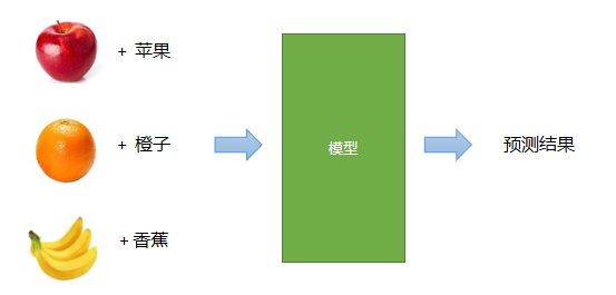
Supervised learning

The learning method of training the model with known data output (labeled) and adjusting and optimizing according to the output is called supervised learning

Unsupervised learning

When there is no known output, the classification is carried out only according to the correlation of input information

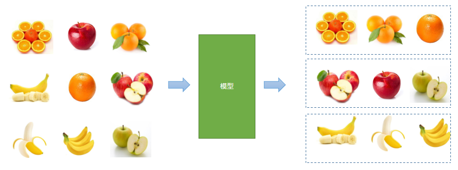
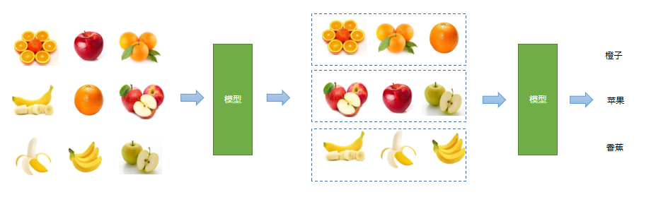
Semi supervision

Firstly, the categories are divided by unsupervised learning, and then the output is predicted by supervised learning For example, cluster similar fruits first, and then identify which category they are

Reinforcement learning

By rewarding and punishing different decision-making results, the machine learning system tends to be closer to the output of the expected result after long enough training

Batch learning, incremental learning

Batch learning

Separate the learning process from the application process, train the model with all the training data, and then make prediction in the application scenario. When the prediction result is not ideal, return to the learning process and cycle like this

incremental learning

Unify the learning process and application process, and learn new contents in an incremental way while applying, while training and predicting

Model based learning and case-based learning

Model based learning

According to the sample data, a mathematical model is established to connect the output and the output, and the input to be predicted is brought into the model to predict its results For example, there are the following input-output relationships:

According to the data, the model y=2x is obtained

Forecast: when inputting 9, what is the output?

Case based learning

According to past experience, find the sample closest to the input to be predicted and take its output as the prediction result (find the answer from the data center) For example, there is the following set of data:

Forecast: undergraduate, 3, male = = > salary?

General process of machine learning (key points)

1. Data collection means, such as manual collection, automatic equipment collection, crawler, etc
2. Data cleaning: clean up the data with standard data, large error and meaningless data

​ Note: the above is called data processing, including data retrieval, data mining, crawler

1. Select model (algorithm)
2. Training model
3. Model evaluation
4. test model

​ Note: steps 3 ~ 6 are mainly the machine learning process, including algorithms, frameworks, tools, etc

1. Application model
2. Model maintenance

Typical applications of machine learning

1. Stock price forecast
2. Recommendation engine
3. natural language processing
4. Speech processing: speech recognition, speech synthesis
5. Image recognition, face recognition
6. ......

Basic problems of machine learning (key points)

Regression problem

According to the known input and output, find a model with the best performance, and substitute the input of unknown output into the model to obtain continuous output For example:

• Predict the house price according to the house area, location, construction age and other conditions
• Predict the price of a stock according to various external conditions
• Prediction of grain harvest based on agricultural and meteorological data
• Calculate the similarity of two faces

classification problem

According to the known inputs and outputs, find the model with the best performance, and bring the inputs of unknown outputs into the model to obtain discrete outputs, such as:

• Handwriting recognition (10 category classification problems)
• Fruit, flowers, animal identification
• Defect detection of industrial products (second classification of good and defective products)
• Identify the emotions expressed in a sentence (positive, negative, neutral)

Clustering problem

According to the similarity of known inputs, they are divided into different communities, such as:

• According to the data of a batch of wheat grains, judge which belong to the same variety
• Judge which customers are interested in a product according to their browsing and purchase history on the e-commerce website
• Determine which customers have higher similarity

Dimensionality reduction problem

When the performance loss is as small as possible, reducing the complexity of data and reducing the size of data are called dimensionality reduction problems

Course content

Data preprocessing

Purpose of data preprocessing

1) Remove invalid data, non-standard data and wrong data

2) Make up the missing value

3) Unified processing of data range, dimension, format and type makes subsequent calculation easier

Pretreatment method

Standardization (mean removal)

Let the average value of each column in the sample matrix be 0 and the standard deviation be 1 If there are three numbers a, B and C, the average value is:

m=(a+b+c)/3

a′=a−m

b′=b−m

The average value after pretreatment is 0:

(a′+b′+c′)/3=((a+b+c)−3m)/3=0

Standard deviation after pretreatment: s=sqrt(((a − m)2+(b − m)2+(c − m)2)/3)

a′′=a/s

b′′=b/s

c'' = c / s

s′′=sqrt(((a′/s)2+(b′/s)2+(c′/s)2)/3)

=sqrt((a' ^ 2 + b' ^ 2 + c' ^ 2) / (3 *s ^2))

=1

Standard deviation: also known as mean square deviation, it is the square root of the arithmetic mean of the square of the deviation from the mean σ Indicates that the standard deviation can reflect the dispersion of a data set

Code example:

# Data preprocessing: mean removal example
import numpy as np
import sklearn.preprocessing as sp

# sample data 
raw_samples = np.array([
    [3.0, -1.0, 2.0],
    [0.0, 4.0, 3.0],
    [1.0, -4.0, 2.0]
])
print(raw_samples)
print(raw_samples.mean(axis=0))  # Average each column
print(raw_samples.std(axis=0))  # Calculate the standard deviation of each column

std_samples = raw_samples.copy()  # Copy sample data
for col in std_samples.T:  # Traverse each column
    col_mean = col.mean()  # Calculate average
    col_std = col.std()  # Standard deviation
    col -= col_mean  # Minus average
    col /= col_std  # Divide by standard deviation

print(std_samples)
print(std_samples.mean(axis=0))
print(std_samples.std(axis=0))

We can also use the sp.scale function provided by sklearn to realize the same function, as shown in the following code:

std_samples = sp.scale(raw_samples) # Standard removal
print(std_samples)
print(std_samples.mean(axis=0))
print(std_samples.std(axis=0))

Range scaling

Set the minimum and maximum values of each column in the sample matrix as the same interval to unify the range of each eigenvalue If there are three numbers a, b and c, where b is the minimum value and c is the maximum value, then:

a′=a−b

b′=b−b

c′=c−b

The scaling calculation method is as follows:

a′′=a′/c′

b′′=b′/c′

c′′=c′/c′

After calculation, the minimum value is 0 and the maximum value is 1 The following is an example of range scaling

# Data preprocessing: range scaling
import numpy as np
import sklearn.preprocessing as sp

# sample data 
raw_samples = np.array([
    [1.0, 2.0, 3.0],
    [4.0, 5.0, 6.0],
    [7.0, 8.0, 9.0]]).astype("float64")

# print(raw_samples)
mms_samples = raw_samples.copy()  # Copy sample data

for col in mms_samples.T:
    col_min = col.min()
    col_max = col.max()
    col -= col_min
    col /= (col_max - col_min)
print(mms_samples)

We can also realize the same function through the object provided by sklearn, as shown in the following code:

# Creates a range scaler object based on a given range
mms = sp.MinMaxScaler(feature_range=(0, 1))# Define the object (modify the scope and observe the phenomenon)
# Use the range scaler to scale the range of eigenvalues
mms_samples = mms.fit_transform(raw_samples) # zoom
print(mms_samples)

Execution result:

[[0.  0.  0. ]
 [0.5 0.5 0.5]
 [1.  1.  1. ]]
[[0.  0.  0. ]
 [0.5 0.5 0.5]
 [1.  1.  1. ]]

normalization

Reflect the proportion of samples Divide each eigenvalue of each sample by the sum of the absolute values of each eigenvalue of the sample For the transformed sample matrix, the sum of the absolute values of the eigenvalues of each sample is 1 For example, in the following sample reflecting the popularity of programming language, compared with 2017, the number of Python developers decreased by 20000, but the proportion did increase:

The sample code of normalization preprocessing is as follows:

# Data preprocessing: normalization
import numpy as np
import sklearn.preprocessing as sp

# sample data 
raw_samples = np.array([
    [10.0, 20.0, 5.0],
    [8.0, 10.0, 1.0]
])
print(raw_samples)
nor_samples = raw_samples.copy()  # Copy sample data

for row in nor_samples:
    row /= abs(row).sum()  # First find the absolute value of the line, then sum it, and then divide it by the sum of the absolute values

print(nor_samples) # Print results

In the sklearn library, you can call sp.normalize() function for normalization. The prototype of the function is:

sp.normalize(Original sample, norm='l2')
# l1: l1 norm, divided by the sum of the absolute values of each element in the vector
# l2: l2 norm, divided by the sum of the squares of the elements in the vector

Use the normalization processing code in the sklearn library as indicated below:

nor_samples = sp.normalize(raw_samples, norm='l1')
print(nor_samples) # Print results

Binarization

According to a preset threshold, 0 and 1 are used to indicate whether the eigenvalue exceeds the threshold The following is the code to realize binarization preprocessing:

# Binarization
import numpy as np
import sklearn.preprocessing as sp

raw_samples = np.array([[65.5, 89.0, 73.0],
                        [55.0, 99.0, 98.5],
                        [45.0, 22.5, 60.0]])
bin_samples = raw_samples.copy()  # Copy array
# Generate mask array
mask1 = bin_samples < 60
mask2 = bin_samples >= 60
# Binarization through mask
bin_samples[mask1] = 0
bin_samples[mask2] = 1

print(bin_samples)  # Print results

Similarly, you can also use the sklearn library to process:

bin = sp.Binarizer(threshold=59) # Create binarized objects (note boundary values)
bin_samples = bin.transform(raw_samples) # Binarization pretreatment
print(bin_samples)

Binary coding will lead to information loss, which is an irreversible numerical conversion In case of reversible conversion, heat only coding is required

Unique heat coding

According to the number of feature median, a sequence composed of one 1 and several zeros is established to encode all feature values For example, there are the following samples:

\left[ \begin{matrix} 1 & 3 & 2\\ 7 & 5 & 4\\ 1 & 8 & 6\\ 7 & 3 & 9\\ \end{matrix} \right]

For the first column, there are two values, 1 encoded with 10 and 7 encoded with 01

For the second column, there are three values. 3 uses 100 code, 5 uses 010 code, and 8 uses 001 code

For the third column, there are four values. 2 uses 1000 code, 4 uses 0100 code, 6 uses 0010 code and 9 uses 0001 code

The coding field is coded according to the number of eigenvalues and distinguished by position The result of the heat independent coding is:

\left[ \begin{matrix} 10 & 100 & 1000\\ 01 & 010 & 0100\\ 10 & 001 & 0010\\ 01 & 100 & 0001\\ \end{matrix} \right]

The codes for exclusive coding using the functions provided by sklearn library are as follows:

# Single heat coding example
import numpy as np
import sklearn.preprocessing as sp

raw_samples = np.array([[1, 3, 2],
                        [7, 5, 4],
                        [1, 8, 6],
                        [7, 3, 9]])

one_hot_encoder = sp.OneHotEncoder(
    sparse=False, # Sparse format
    dtype="int32",
    categories="auto")# Automatic coding
oh_samples = one_hot_encoder.fit_transform(raw_samples) # Perform heat only coding
print(oh_samples)

print(one_hot_encoder.inverse_transform(oh_samples)) # decode

Execution result:

[[1 0 1 0 0 1 0 0 0]
 [0 1 0 1 0 0 1 0 0]
 [1 0 0 0 1 0 0 1 0]
 [0 1 1 0 0 0 0 0 1]]
 
[[1 3 2]
 [7 5 4]
 [1 8 6]
 [7 3 9]]

Tag code

According to the position of the string eigenvalue in the feature sequence, a digital label is assigned to it, which is used to provide it to the learning model based on numerical algorithm The code is as follows:

# Tag code
import numpy as np
import sklearn.preprocessing as sp

raw_samples = np.array(['audi', 'ford', 'audi',
                        'bmw','ford', 'bmw'])

lb_encoder = sp.LabelEncoder() # Define label coding object
lb_samples = lb_encoder.fit_transform(raw_samples) # Execute tag encoding
print(lb_samples)

print(lb_encoder.inverse_transform(lb_samples)) # Reverse conversion

Execution result:

[0 2 0 1 2 1]
['audi' 'ford' 'audi' 'bmw' 'ford' 'bmw']