Machine learning practice: handwritten numeral recognition
1. Experimental description
-
In this experiment, we will use the k-nearest neighbor algorithm to recognize handwritten digits, build the k-nearest neighbor algorithm function through the python command line, input the data provided by the experiment, classify the data, and view the classification results and error rate. Through the study of this experiment, we will master the basic principle and classification process of k-nearest neighbor algorithm
-
Experiment duration: 45 minutes
-
Main steps:
-
Data preparation
-
Anaconda environment deployment
-
Write text conversion vector function
-
Write k-nearest neighbor classifier function
-
Write and call test functions
-
2. Experimental environment
-
Number of virtual machines: 1
-
System version: CentOS 7.5
-
Python 3.5
3. Related skills
- Python Programming
- Anaconda use
- k-nearest neighbor classification algorithm
4. Relevant knowledge points
-
Parsing and importing data from text files
-
k nn
5. Realization effect
- Print the classification data and error rate results of each data file, as shown in the following figure

6. Experimental steps
6.1 preparation
6.1.1 preparing data sets
6.1.2 copy and decompress data
[zkpk@master ~]$ cd experiment/KNN
[zkpk@master KNN]$ unzip digit.zip
6.1.3 data introduction: after decompression, there are two folders in the digits directory, namely:
6.1.3.1 trainingdigits: training data, 1935 files, about 200 files for each number.
6.1.3.2 testdigits: test data, 947 files, about 100 files for each number.
[zkpk@master KNN]$ cd digits
[zkpk@master digits]$ ls

6.1.3.3 store a handwritten number in each file. The file name is similar to ` 0_7.txt `, the first number '0' means that the handwritten number in the file is 0, and the subsequent '7' is the serial number.
6.1.3.4 we use the data in the directory trainingDigits to train the classifier, and use the data in the directory testDigits to test the effect of the classifier. The two sets of data do not overlap. You can check whether the files in these folders meet the requirements. Based on these data, we begin to implement KNN algorithm.
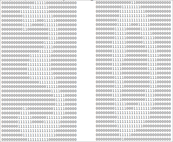
6.1.3.5 the data is originally 32 * 32 black-and-white picture data. Here, for convenience of understanding, we provide data in text format converted from images, as follows:
6.2 installation and deployment of Anaconda environment
6.2.1Anaconda is a python distribution for scientific computing. It supports Linux, MAC and windows systems and provides the functions of package management and environment management. It can easily solve the problems of coexistence and switching of multiple versions of Python and installation of various third-party packages. Anaconda uses the tool / command conda to manage the package and environment, and has included Python and related supporting tools
6.2.2 switch to root (with zkpk password) and install Anaconda package, which depends on bzip2 package. If you confirm that it has been installed, you can skip this step
[zkpk@master digits]$ cd
[zkpk@master ~]$ su
[root@master zkpk]$ yum install -y bzip2
6.2.3 go back to zkpk user and copy Anaconda software package from public directory to zkpk home directory
[root@master zkpk]$ exit
[zkpk@master ~]$ cd /home/zkpk/tgz
[zkpk@master tgz]$ pwd
/home/zkpk/tgz
[zkpk@master tgz]$ cp Anaconda3-4.0.0-Linux-x86_64.sh  ~/
[zkpk@master tgz]$ cd

6.2.4 installing and deploying using commands
6.2.4.1 install Anaconda with bash. After seeing the following prompt, press enter to continue
[zkpk@master ~]$ bash Anaconda3-4.0.0-Linux-x86_64.sh

6.2.4.2 enter yes in the license interface

6.2.4.3 when you see the following prompt, continue to enter to confirm, specify the installation directory and start the installation

6.2.4.4 after installation, you will be prompted to configure Anaconda's environment variables. Enter yes

6.2.4.5 make the added environment variables effective
[zkpk@master ~]$ source ~/.bashrc
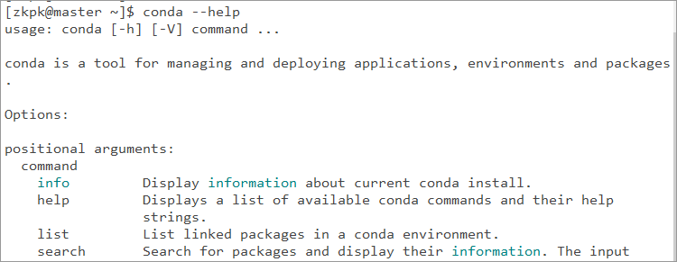
6.2.4.6 verify that the installation is successful
6.2.4.7 it is necessary to configure the download source of relevant packages here. We configure the domestic image source to speed up the download of software; Execute the following commands
[zkpk@master ~]$conda config --add channels https://mirrors.tuna.tsinghua.edu.cn/anaconda/pkgs/main/
[zkpk@master ~]$conda config --add channels https://mirrors.tuna.tsinghua.edu.cn/anaconda/pkgs/free/
[zkpk@master ~]$conda config --set show_channel_urls yes
6.2.4.8 create a virtual environment for the experiment. Use the following command to create a python 3.0 named "zkbc" 5 virtual environment
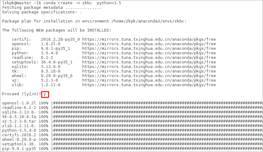
[zkpk@master ~]$ conda create -n zkbc python=3.5
6.2.4.9 the terminal will ask whether to install dependency, and enter y to start installation
6.2.4.10 when we enter the virtual environment, we enter a python environment isolated from the native environment
[zkpk@master ~]$ source activate zkbc
6.2.4.11 how to exit a virtual environment
(zkbc) [zkpk@master ~]$ source deactivate
6.3 start coding
6.3.1 entering the virtual environment
[zkpk@master ~]$ source activate zkbc
6.3.2 use conda to install the installation package required for the experiment. During the installation, enter y to continue the installation. After the installation is completed, enter the python command line; During installation, enter y to continue the installation
(zkbc)[zkpk@master ~]$ conda install numpy
(zkbc)[zkpk@master ~]$ python
6.3.3 import the relevant packages required for the experiment
>>>from os import listdir
>>>import operator
>>>import numpy as np
6.3.4 we customize a function tovector that processes data into a vector. This function first creates a 1 * 1024 Numpy array returnvector, then opens the data file under the specified file path, reads the first 32 rows of the file circularly, and stores the values of the first 32 columns of each row in the array returnvector, In fact, here is to convert each data file into a vector. (after the method is written, press enter twice to exit the method writing and continue to write the following code)
>>>def tovector(filename):
...    # Create vector
...    returnVect = np.zeros((1,1024))
...    # Open the data file and read the contents of each line
...    fr = open(filename)
...    for i in range(32):	# Because there are 32 lines in the file
...        # Read each line
...        lineStr = fr.readline()
...        # Convert the first 32 characters of each line into int and store it in the vector
...        for j in range(32):	# Because each line of the file has 32 characters in total
...            returnVect[0,32*i+j] = int(lineStr[j])
...    return returnVect

6.3.5 the core of KNN algorithm is to calculate the "distance". Here we define the KNN algorithm implementation function KNNAlg, and the parameters of the function include:
6.3.5.1 inputvector: input vector used for classification
6.3.5.2trainDataSet: input training sample set
6.3.5.3 labels: class label vector of sample data
6.3.5.4k: used to select the number of nearest neighbors
6.3.6 algorithm implementation process:
6.3.6.1 calculate the distance between the point in the known category dataset and the current point;
6.3.6.2 sort according to the order of increasing distance;
6.3.6.3 select k points with the minimum distance from the current point;
6.3.6.4 determine the occurrence frequency of the category of the first k points;
6.3.6.5 return the category with the highest frequency of the first k points as the prediction classification of the current point
>>>def KnnAlg(inputvector, trainDataSet, labels, k):
...    # Quantity of sample data obtained
...    trainDataSize = trainDataSet.shape[0]
...    # Matrix operation to calculate the difference between the test data and the corresponding data items of each sample data
...    diffMat = np.tile(inputvector, (trainDataSize,1)) - trainDataSet
...    # sqDistances sum of squares of the results of the previous step
...    sqDiffMat = diffMat**2
...    sqDistances = sqDiffMat.sum(axis=1)
...    # Take the square root to get the distance vector
...    distances = sqDistances**0.5
...    # Sort from low to high according to the distance, and return the index of the corresponding element
...    sortedDistIndicies = distances.argsort()
...    classCount={}
...    # Take out the latest sample data in turn
...    for i in range(k):
...        # Record the category of the sample data
...        voteIlabel = labels[sortedDistIndicies[i]]
...        classCount[voteIlabel] = classCount.get(voteIlabel,0) + 1
...    # Sort the frequency of categories from high to low
...    sortedClassCount = sorted(classCount.items(), key=operator.itemgetter(1), reverse=True)
...    # Returns the most frequent category
...    return sortedClassCount[0][0]

6.3.7 test algorithm: use k-nearest neighbor algorithm to recognize handwritten digits
6.3.8 we have defined the function that can recognize the data processing component classer. Next, we define the test function handwritingClassTest to read the data file, input the data into the processing function, and then input it into the classifier function to detect the execution effect of the classifier
6.3.9 steps of test function:
6.3.9.1 read the training data (handwritten picture data) to the vector, and extract the category label list (the real number corresponding to each vector) from the data file name
6.3.9.2 read the test data to the vector and extract the category label from the data file name
6.3.9.3 execute KNN algorithm to test the test data and obtain the classification results
6.3.9.4 compare with the actual category label and record the classification error rate
6.3.9.5 print the classified data and error rate of each data file as the final result
>>>def handwritingClassTest():
...    # Defines a list of class labels for sample data
...    hwLabels = []
...    # Read training data file list
...    trainingFileList = listdir('/home/zkpk/experiment/KNN/digits/trainingDigits')
...    m = len(trainingFileList)
...    # Initialize training data matrix (M*1024)
...    trainingMat = np.zeros((m,1024))
...    # Read all training data to the data matrix in turn
...    for i in range(m):
...        # Extract the number in the file name
...        fileNameStr = trainingFileList[i]
...        fileStr = fileNameStr.split('.')[0]
...        classNumStr = int(fileStr.split('_')[0])
...        hwLabels.append(classNumStr)
...        # Store the training data into the matrix
...        trainingMat[i,:] = tovector('/home/zkpk/experiment/KNN/digits/trainingDigits/%s' % fileNameStr)
...    # Read test data list
...    testFileList = listdir('/home/zkpk/experiment/KNN/digits/testDigits')
...    # Initialization error rate
...    errorCount = 0.0
...    mTest = len(testFileList)
...    # Loop test each test data file
...    for i in range(mTest):
...        # Extract the digital ID in the file name
...        fileNameStr = testFileList[i]
...        fileStr = fileNameStr.split('.')[0]
...        classNumStr = int(fileStr.split('_')[0])
...        # Call the tovector function to extract the data vector
...        vectorUnderTest = tovector('/home/zkpk/experiment/KNN/digits/testDigits/%s' % fileNameStr)
...        # Call the knalg classifier function to classify the test data files
...        classifierResult = KnnAlg(vectorUnderTest, trainingMat, hwLabels, 3)
...        # Print KNN algorithm classification results and real classification results
...        print ("the classifier came back with: %d, the real answer is: %d" %(classifierResult, classNumStr))
...        # Judge whether the result of KNN algorithm is accurate
...        if (classifierResult != classNumStr): errorCount += 1.0
...    # Print error rate
...    print("\nthe total number of errors is: %d" % errorCount)
...    print("\nthe total error rate is: %f" % (errorCount/float(mTest)))
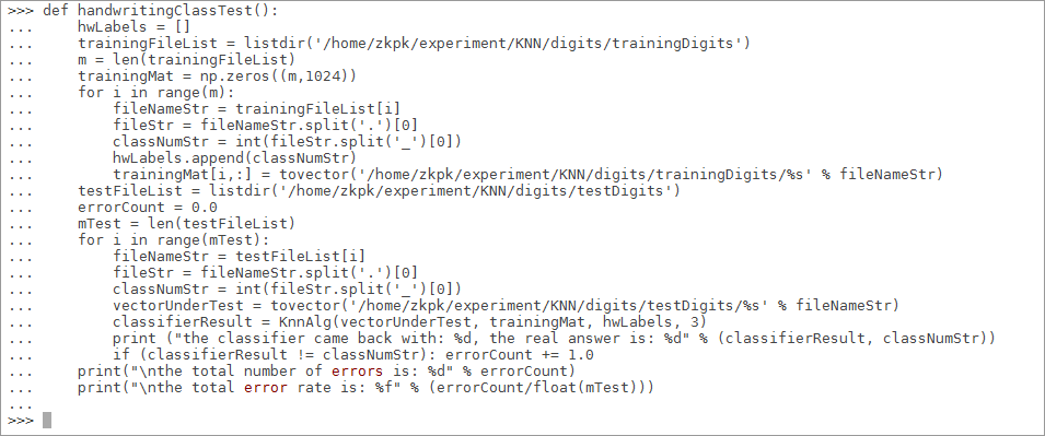
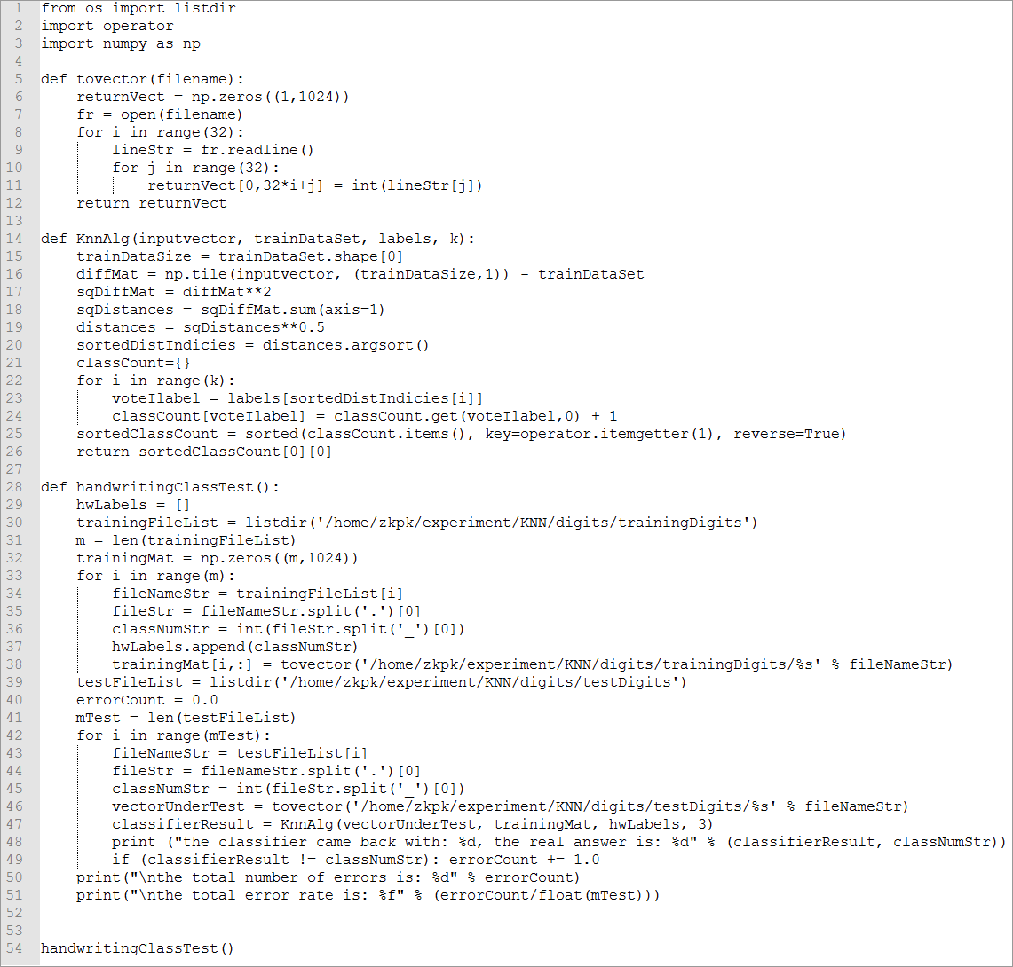
6.3.10 so far, the functions we need to define have been defined, including text conversion vector function tovector, KNN classifier algorithm knalg, and test algorithm handwritingClassTest
6.3.11 finally, we call the test function handwritingClassTest to view the classification results returned by the terminal
>>>handwritingClassTest()
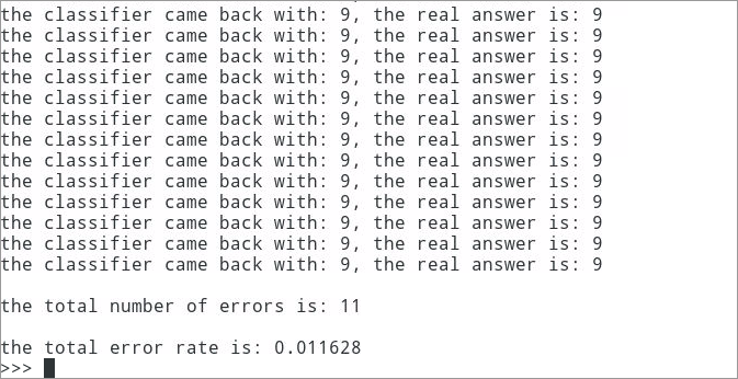
6.3.12 it can be seen that there are 11 classification errors, and the error rate is about 1.16%. This error rate is relatively low. In the k-nearest neighbor algorithm, changing the value of Variable k, modifying the function handwritingClassTest, randomly selecting training samples and changing the number of training samples will have an impact on the error rate of the k-nearest neighbor algorithm. If you are interested, you can change the values of these variables, Observe the change of error rate
7. Reference answer
8. Summary
This experiment uses k-nearest neighbor algorithm to classify and predict the text data converted from handwritten digital pictures. Through this experiment, we should master the basic principle and classification process of k-nearest neighbor algorithm. We can see that the core of k-nearest neighbor algorithm is "distance" calculation, and another key factor affecting classification accuracy is the selection of K value. You can also try to change the given K value in this experiment and compare the classification accuracy under different K values.
There are 11 classification errors, and the error rate is about 1.16%. This error rate is relatively low. In the k-nearest neighbor algorithm, changing the value of Variable k, modifying the function handwritingClassTest, randomly selecting training samples and changing the number of training samples will affect the error rate of the k-nearest neighbor algorithm. If you are interested, you can change the values of these variables and observe the change of the error rate