1, Overview of k-nearest neighbor algorithm

In short, the k-nearest neighbor algorithm uses the method of measuring the distance between different eigenvalues for classification.

k-nearest neighbor
Advantages: high precision, insensitive to outliers and no data input assumption.
Disadvantages: high computational complexity and space complexity.
Applicable data range: numerical type and nominal type.

The working principle of k-nearest neighbor algorithm (kNN) is that there is a sample data set, also known as training sample set, and each data in the sample set has a label, that is, we know the corresponding relationship between each data in the sample set and its classification. After entering the new data without labels, each feature of the new data is compared with the corresponding feature of the data in the sample set, and then the algorithm extracts the classification label of the data with the most similar feature (nearest neighbor) in the sample set. Finally, the most frequent classification among the k most similar data is selected as the classification of new data.

Generally speaking, only the first k most similar data in the sample data set are selected, which is the source of K in the k-nearest neighbor algorithm. Generally, K is an integer not greater than 20.

General flow of k-nearest neighbor algorithm
(1) Collect data: any method can be used.
(2) Prepare data: the value required for distance calculation, preferably in a structured data format.
(3) Analyze data: any method can be used.
(4) Training algorithm: this step is not applicable to k-nearest neighbor algorithm.
(5) Test algorithm: calculate the error rate.
(6) Using the algorithm: first, input the sample data and structured output results, then run the k-nearest neighbor algorithm to determine which classification the input data belongs to respectively, and finally perform subsequent processing on the calculated classification.

1. Preparation: import data using Python

Create a Python module named kNN.py and write the following code

import numpy as np

'''
Parameters:
    nothing
Returns:
    group - data set
	labels - Classification label
'''

# Function Description: create dataset
def createDataSet():
    # Four sets of 2D features
    group = np.array([[1.0, 1.1], [1.0, 1.0], [0, 0], [0, 0.1]])
    # Labels for four sets of features
    labels = ['A', 'A', 'B', 'B']
    return group, labels

if __name__ == '__main__':
    group, labels = createDataSet()
    print(group)
    print(labels)

>>>
[[1.  1.1]
 [1.  1. ]
 [0.  0. ]
 [0.  0.1]]
['A', 'A', 'B', 'B']

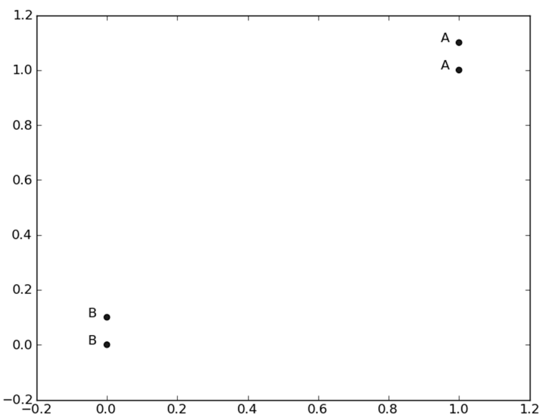
There are four groups of data, and each group of data has two known attributes or eigenvalues. Each row of the group matrix above contains a different data. We can think of it as a different measurement point or entry in a log file. Due to the limitation of human brain, we can only visually process transactions below three dimensions. Therefore, in order to simply realize data visualization, only two features are usually used for each data point.
Vector labels contains the label information of each data point. The number of elements contained in labels is equal to the number of rows of the group matrix. Here, the data point (1, 1.1) is defined as class A, and the data point (0, 0.1) is defined as class B

2. Parse data from text file

For each point in the dataset with unknown category attributes, do the following in turn:
(1) Calculating the distance between the point in the known category dataset and the current point;
(2) Sort by increasing distance;
(3) Select the k points with the minimum distance from the current point;
(4) Determine the occurrence frequency of the category where the first k points are located;
(5) Return the category with the highest frequency of the first k points as the prediction classification of the current point.

According to the two-point distance formula (Euclidean distance formula), calculate the distance between two vector points xA and xB.

d = ( x A 0 − x B 0 ) 2 + ( x A 1 − x B 1 ) 2 d = \sqrt {(xA_0 - xB_0)^2 + (xA_1 - xB_1)^2} d=(xA0​−xB0​)2+(xA1​−xB1​)2 ​

Next, sort the data from small to large. Select the first k points with the smallest distance and return the classification results

'''
Parameters:
    inX - Data for classification(Test set)
    dataSet - Data for training(Training set)
    labes - Classification label
    k - kNN Algorithm parameters,Select the one with the smallest distance k Points
Returns:
    sortedClassCount[0][0] - Classification results
'''

# Function Description: kNN algorithm, classifier
def classify0(inX, dataSet, labels, k):
    # numpy function shape[0] returns the number of rows of dataSet
    dataSetSize = dataSet.shape[0]
    # Repeat inX once in the direction of column vector (horizontal), and inX times in the direction of row vector (vertical)
    diffMat = np.tile(inX, (dataSetSize, 1)) - dataSet
    # Square of two-dimensional feature subtraction
    sqDiffMat = diffMat**2
    # sum() adds all elements, sum(0) columns, and sum(1) rows
    sqDistances = sqDiffMat.sum(axis=1)
    # Square off and calculate the distance
    distances = sqDistances**0.5
    # Returns the index value of the elements in distances sorted from small to large
    sortedDistIndicies = distances.argsort()
    # A dictionary that records the number of times a category
    classCount = {}
    for i in range(k):
        # Take out the category of the first k elements
        voteIlabel = labels[sortedDistIndicies[i]]
        # dict.get(key,default=None), the get() method of the dictionary, returns the value of the specified key. If the value is not in the field, it returns the default value
        # Calculate category times
        classCount[voteIlabel] = classCount.get(voteIlabel, 0) + 1
    # items() in Python 3 replaces itemtems ()
    # Key = operator. Itemsetter (1) sorts according to the values of the dictionary
    # Key = operator.itemsetter (0) sorts according to the key of the dictionary
    # reverse descending sort dictionary
    sortedClassCount = sorted(classCount.items(), key=operator.itemgetter(1), reverse=True)
    # The category that returns the most times, that is, the category to be classified
    return sortedClassCount[0][0]

if __name__ == '__main__':
    group, labels = createDataSet()
    test = [0, 0]
    test_class = classify0(test, group, labels, 3)
    print(test_class)

>>>
B

3. How to test classifiers

"Under what circumstances will the classifier make mistakes?" or "is the answer always correct?" the answer is No. the classifier will not get 100% correct results. We can use a variety of methods to detect the accuracy of the classifier. In addition, the performance of classifier is also affected by many factors, such as classifier setting and data set. In addition, different algorithms may perform completely differently on different data sets.

In order to test the effect of the classifier, we can use the data with known answers. Of course, the answers can not be told to the classifier to test whether the results given by the classifier meet the expected results. Through a large number of test data, we can get the error rate of the classifier - the number of wrong results given by the classifier divided by the total number of test executions. Error rate is a common evaluation method, which is mainly used to evaluate the execution effect of classifier on a data set. The error rate of the perfect classifier is 0, and the error rate of the worst classifier is 1.0. At the same time, it is not difficult to find that the k-nearest neighbor algorithm does not train the data, and directly uses the unknown data to compare with the known data to get the results. Therefore, it can be said that the k-nearest neighbor algorithm does not have an explicit learning process.

2, Using k-nearest neighbor algorithm to improve the pairing effect of dating websites

Using k-nearest neighbor algorithm on dating websites
(1) Collect data: provide text files.
(2) Prepare data: parse text files using Python.
(3) Analysis of data: draw a two-dimensional diffusion diagram using Matplotlib.
(4) Training algorithm: this step is not applicable to k-nearest neighbor algorithm.
(5) Test algorithm: use some data provided by Helen as test samples. The difference between test samples and non test samples is that test samples are classified data. If the predicted classification is different from the actual classification, it will be marked as an error.
(6) Using the algorithm: generate a simple command-line program, and then Helen can input some characteristic data to judge whether the other party is his favorite type.

1. Prepare data: parse data from text files

Preparing data: parsing data from a text file
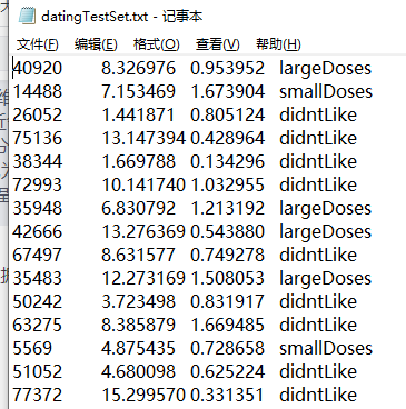
Helen has been collecting dating data for some time. She stores these data in the text file datingTestSet.txt. Each sample data occupies one line, a total of 1000 lines. Helen's sample mainly contains the following three characteristics:

• Frequent flyer miles per year
• Percentage of time spent playing video games
• Litres of ice cream consumed per week

There are three types of tags in the data: largeDoses, smallDoses, and didntLike

Before inputting the above feature data into the classifier, the format of the data to be processed must be changed to the format that the classifier can receive. The data is classified into two parts, namely, the feature matrix and the corresponding classification label vector. Create a function called file2matrix in kNN.py to handle the input format problem. The input of this function is the file name string, and the output is the training sample matrix and class label vector.

'''
Parameters:
    filename - file name
Returns:
    returnMat - Characteristic matrix
    classLabelVector - classification Label vector
'''

# Function Description: open and parse the file to classify the data: 1 means' didntLike 'doesn't like it, 2 means' smallDoses' is generally attractive, and 3 means' largeDoses' is extremely attractive
def file2matrix(filename):
    # Open file
    fr = open(filename)
    # Read all contents of the file
    arrayOLines = fr.readlines()
    # Get the number of file lines
    numberOfLines = len(arrayOLines)
    # Returned NumPy matrix, parsed data: numberOfLines row, 3 columns
    returnMat = np.zeros((numberOfLines, 3))
    # Returned category label vector
    classLabelVector = []
    # Index value of row
    index = 0
    for line in arrayOLines:
        # s.strip(rm). When rm is empty, the blank characters (including '\ n','\r','\t', ') are deleted by default
        line = line.strip()
        # Use s.split(str="",num=string,cout(str)) to slice the string according to the '\ t' separator.
        listFromLine = line.split('\t')
        # The first three columns of data are extracted and stored in the NumPy matrix of returnMat, that is, the characteristic matrix
        returnMat[index, :] = listFromLine[0:3]
        # According to the degree of liking marked in the text, 1 represents dislike, 2 represents general charm and 3 represents great charm
        if listFromLine[-1] == 'didntLike':
            classLabelVector.append(1)
        elif listFromLine[-1] == 'smallDoses':
            classLabelVector.append(2)
        elif listFromLine[-1] == 'largeDoses':
            classLabelVector.append(3)
        index += 1
    return returnMat, classLabelVector

if __name__ == '__main__':
    filename = "datingTestSet.txt"
    datingDataMat, datingLabels = file2matrix(filename)
    print(datingDataMat)
    print(datingLabels)

>>>
[[4.0920000e+04 8.3269760e+00 9.5395200e-01]
 [1.4488000e+04 7.1534690e+00 1.6739040e+00]
 [2.6052000e+04 1.4418710e+00 8.0512400e-01]
 ...
 [2.6575000e+04 1.0650102e+01 8.6662700e-01]
 [4.8111000e+04 9.1345280e+00 7.2804500e-01]
 [4.3757000e+04 7.8826010e+00 1.3324460e+00]]
[3, 2, 1, 1, 1, 1, 3, 3, 1, 3, 1, 1, 2, 1, 1, 1, 1, 1, 2, 3, 2, 1, 2, 3, 2, 3, 2, 3, 2, 1, 3, 1, 3, 1, 2, 1, 1, 2, 3, 3, 1, 2, 3, 3, 3, 1, 1, 1, 1, 2, 2, 1, 3, 2, 2, 2, 2, 3, 1, 2, 1, 2, 2, 2, 2, 2, 3, 2, 3, 1, 2, 3, 2, 2, 1, 3, 1, 1, 3, 3, 1, 2, 3, 1, 3, 1, 2, 2, 1, 1, 3, 3, 1, 2, 1, 3, 3, 2, 1, 1, 3, 1, 2, 3, 3, 2, 3, 3, 1, 2, 3, 2, 1, 3, 1, 2, 1, 1, 2, 3, 2, 3, 2, 3, 2, 1, 3, 3, 3, 1, 3, 2, 2, 3, 1, 3, 3, 3, 1, 3, 1, 1, 3, 3, 2, 3, 3, 1, 2, 3, 2, 2, 3, 3, 3, 1, 2, 2, 1, 1, 3, 2, 3, 3, 1, 2, 1, 3, 1, 2, 3, 2, 3, 1, 1, 1, 3, 2, 3, 1, 3, 2, 1, 3, 2, 2, 3, 2, 3, 2, 1, 1, 3, 1, 3, 2, 2, 2, 3, 2, 2, 1, 2, 2, 3, 1, 3, 3, 2, 1, 1, 1, 2, 1, 3, 3, 3, 3, 2, 1, 1, 1, 2, 3, 2, 1, 3, 1, 3, 2, 2, 3, 1, 3, 1, 1, 2, 1, 2, 2, 1, 3, 1, 3, 2, 3, 1, 2, 3, 1, 1, 1, 1, 2, 3, 2, 2, 3, 1, 2, 1, 1, 1, 3, 3, 2, 1, 1, 1, 2, 2, 3, 1, 1, 1, 2, 1, 1, 2, 1, 1, 1, 2, 2, 3, 2, 3, 3, 3, 3, 1, 2, 3, 1, 1, 1, 3, 1, 3, 2, 2, 1, 3, 1, 3, 2, 2, 1, 2, 2, 3, 1, 3, 2, 1, 1, 3, 3, 2, 3, 3, 2, 3, 1, 3, 1, 3, 3, 1, 3, 2, 1, 3, 1, 3, 2, 1, 2, 2, 1, 3, 1, 1, 3, 3, 2, 2, 3, 1, 2, 3, 3, 2, 2, 1, 1, 1, 1, 3, 2, 1, 1, 3, 2, 1, 1, 3, 3, 3, 2, 3, 2, 1, 1, 1, 1, 1, 3, 2, 2, 1, 2, 1, 3, 2, 1, 3, 2, 1, 3, 1, 1, 3, 3, 3, 3, 2, 1, 1, 2, 1, 3, 3, 2, 1, 2, 3, 2, 1, 2, 2, 2, 1, 1, 3, 1, 1, 2, 3, 1, 1, 2, 3, 1, 3, 1, 1, 2, 2, 1, 2, 2, 2, 3, 1, 1, 1, 3, 1, 3, 1, 3, 3, 1, 1, 1, 3, 2, 3, 3, 2, 2, 1, 1, 1, 2, 1, 2, 2, 3, 3, 3, 1, 1, 3, 3, 2, 3, 3, 2, 3, 3, 3, 2, 3, 3, 1, 2, 3, 2, 1, 1, 1, 1, 3, 3, 3, 3, 2, 1, 1, 1, 1, 3, 1, 1, 2, 1, 1, 2, 3, 2, 1, 2, 2, 2, 3, 2, 1, 3, 2, 3, 2, 3, 2, 1, 1, 2, 3, 1, 3, 3, 3, 1, 2, 1, 2, 2, 1, 2, 2, 2, 2, 2, 3, 2, 1, 3, 3, 2, 2, 2, 3, 1, 2, 1, 1, 3, 2, 3, 2, 3, 2, 3, 3, 2, 2, 1, 3, 1, 2, 1, 3, 1, 1, 1, 3, 1, 1, 3, 3, 2, 2, 1, 3, 1, 1, 3, 2, 3, 1, 1, 3, 1, 3, 3, 1, 2, 3, 1, 3, 1, 1, 2, 1, 3, 1, 1, 1, 1, 2, 1, 3, 1, 2, 1, 3, 1, 3, 1, 1, 2, 2, 2, 3, 2, 2, 1, 2, 3, 3, 2, 3, 3, 3, 2, 3, 3, 1, 3, 2, 3, 2, 1, 2, 1, 1, 1, 2, 3, 2, 2, 1, 2, 2, 1, 3, 1, 3, 3, 3, 2, 2, 3, 3, 1, 2, 2, 2, 3, 1, 2, 1, 3, 1, 2, 3, 1, 1, 1, 2, 2, 3, 1, 3, 1, 1, 3, 1, 2, 3, 1, 2, 3, 1, 2, 3, 2, 2, 2, 3, 1, 3, 1, 2, 3, 2, 2, 3, 1, 2, 3, 2, 3, 1, 2, 2, 3, 1, 1, 1, 2, 2, 1, 1, 2, 1, 2, 1, 2, 3, 2, 1, 3, 3, 3, 1, 1, 3, 1, 2, 3, 3, 2, 2, 2, 1, 2, 3, 2, 2, 3, 2, 2, 2, 3, 3, 2, 1, 3, 2, 1, 3, 3, 1, 2, 3, 2, 1, 3, 3, 3, 1, 2, 2, 2, 3, 2, 3, 3, 1, 2, 1, 1, 2, 1, 3, 1, 2, 2, 1, 3, 2, 1, 3, 3, 2, 2, 2, 1, 2, 2, 1, 3, 1, 3, 1, 3, 3, 1, 1, 2, 3, 2, 2, 3, 1, 1, 1, 1, 3, 2, 2, 1, 3, 1, 2, 3, 1, 3, 1, 3, 1, 1, 3, 2, 3, 1, 1, 3, 3, 3, 3, 1, 3, 2, 2, 1, 1, 3, 3, 2, 2, 2, 1, 2, 1, 2, 1, 3, 2, 1, 2, 2, 3, 1, 2, 2, 2, 3, 2, 1, 2, 1, 2, 3, 3, 2, 3, 1, 1, 3, 3, 1, 2, 2, 2, 2, 2, 2, 1, 3, 3, 3, 3, 3, 1, 1, 3, 2, 1, 2, 1, 2, 2, 3, 2, 2, 2, 3, 1, 2, 1, 2, 2, 1, 1, 2, 3, 3, 1, 1, 1, 1, 3, 3, 3, 3, 3, 3, 1, 3, 3, 2, 3, 2, 3, 3, 2, 2, 1, 1, 1, 3, 3, 1, 1, 1, 3, 3, 2, 1, 2, 1, 1, 2, 2, 1, 1, 1, 3, 1, 1, 2, 3, 2, 2, 1, 3, 1, 2, 3, 1, 2, 2, 2, 2, 3, 2, 3, 3, 1, 2, 1, 2, 3, 1, 3, 2, 2, 2, 2, 2, 2, 2, 2, 2, 2, 2, 2, 3, 2, 2, 2, 2, 2, 1, 3, 3, 3]

Above is the characteristic matrix and below is the label vector.

2. Analyze data: use Matplotlib to create scatter chart

Now that the data has been imported from the text file and formatted into the desired format, we need to understand the real meaning of the data. Of course, we can browse text files directly, but this method is very unfriendly. Generally speaking, we will display the data intuitively in a graphical way. Next, use Python tools to graphically display the data content in order to identify some data patterns.

from matplotlib.font_manager import FontProperties
import matplotlib.lines as mlines
import matplotlib.pyplot as plt
import numpy as np

'''
Parameters:
    datingDataMat - Characteristic matrix
    datingLabels - classification Label
Returns:
    nothing
'''

# Function Description: visual data
def showdatas(datingDataMat, datingLabels):
    # Format Chinese characters
    font = FontProperties(fname=r"c:\windows\fonts\simsun.ttc", size=14)
    # The fig canvas is divided into one row and one column. The x-axis and y-axis are not shared. The size of the fig canvas is (13,8)
    # When nrows=2 and ncols=2, the representative fig canvas is divided into four areas, and axs[0][0] represents the first area in the first line
    fig, axs = plt.subplots(nrows=2, ncols=2, sharex=False, sharey=False, figsize=(13, 8))

    numberOfLabels = len(datingLabels)
    LabelsColors = []
    for i in datingLabels:
        if i == 1:
            LabelsColors.append('black')
        if i == 2:
            LabelsColors.append('orange')
        if i == 3:
            LabelsColors.append('red')

    # Draw the scatter diagram, and draw the scatter data with the first column (frequent flyer routine) and the second column (playing games) of the datingDataMat matrix. The scatter size is 15 and the transparency is 0.5
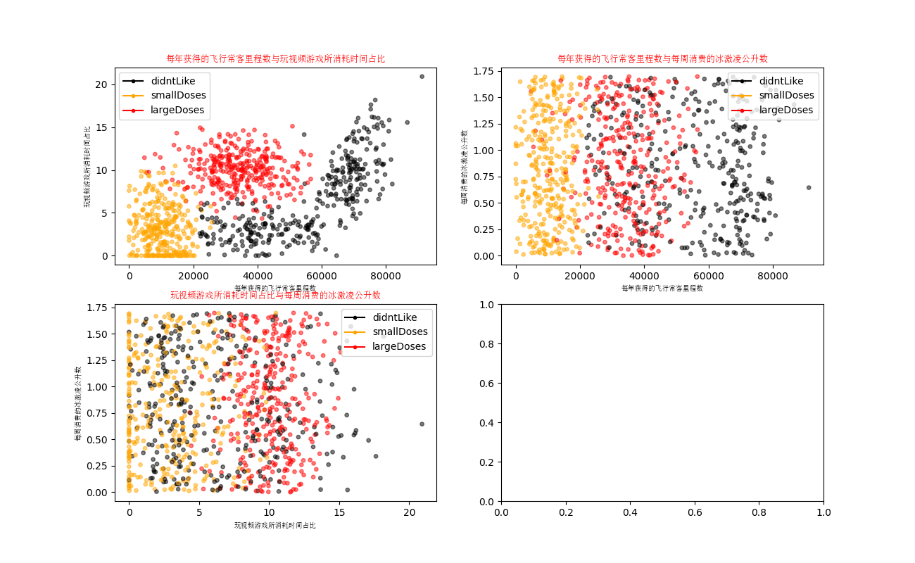
    axs[0][0].scatter(x=datingDataMat[:, 0], y=datingDataMat[:, 1], color=LabelsColors, s=15, alpha=.5)
    # Set title, x-axis label, y-axis label
    axs0_title_text = axs[0][0].set_title(u'Proportion of frequent flyer mileage obtained each year and time spent playing video games', FontProperties=font)
    axs0_xlabel_text = axs[0][0].set_xlabel(u'Frequent flyer miles per year', FontProperties=font)
    axs0_ylabel_text = axs[0][0].set_ylabel(u'Percentage of time spent playing video games', FontProperties=font)
    plt.setp(axs0_title_text, size=9, weight='bold', color='red')
    plt.setp(axs0_xlabel_text, size=7, weight='bold', color='black')
    plt.setp(axs0_ylabel_text, size=7, weight='bold', color='black')

    # Draw the scatter diagram, and draw the scatter data with the first column (frequent flyer routine) and the second column (ice cream) of the datingDataMat matrix. The scatter size is 15 and the transparency is 0.5
    axs[0][1].scatter(x=datingDataMat[:, 0], y=datingDataMat[:, 2], color=LabelsColors, s=15, alpha=.5)
    axs1_title_text = axs[0][1].set_title(u'Frequent flyer miles obtained per year and litres of ice cream consumed per week', FontProperties=font)
    axs1_xlabel_text = axs[0][1].set_xlabel(u'Frequent flyer miles per year', FontProperties=font)
    axs1_ylabel_text = axs[0][1].set_ylabel(u'Litres of ice cream consumed per week', FontProperties=font)
    plt.setp(axs1_title_text, size=9, weight='bold', color='red')
    plt.setp(axs1_xlabel_text, size=7, weight='bold', color='black')
    plt.setp(axs1_ylabel_text, size=7, weight='bold', color='black')

    # Draw the scatter diagram, and draw the scatter data with the first column (playing games) and the second column (ice cream) of the datingDataMat matrix. The scatter size is 15 and the transparency is 0.5
    axs[1][0].scatter(x=datingDataMat[:, 1], y=datingDataMat[:, 2], color=LabelsColors, s=15, alpha=.5)
    axs2_title_text = axs[1][0].set_title(u'Proportion of time spent playing video games and litres of ice cream consumed per week', FontProperties=font)
    axs2_xlabel_text = axs[1][0].set_xlabel(u'Percentage of time spent playing video games', FontProperties=font)
    axs2_ylabel_text = axs[1][0].set_ylabel(u'Litres of ice cream consumed per week', FontProperties=font)
    plt.setp(axs2_title_text, size=9, weight='bold', color='red')
    plt.setp(axs2_xlabel_text, size=7, weight='bold', color='black')
    plt.setp(axs2_ylabel_text, size=7, weight='bold', color='black')

    # Set legend
    didntLike = mlines.Line2D([], [], color='black', marker='.', markersize=6, label='didntLike')
    smallDoses  = mlines.Line2D([], [], color='orange', marker='.', markersize=6, label='smallDoses')
    largeDoses  = mlines.Line2D([], [], color='red', marker='.', markersize=6, label='largeDoses')

    # Add legend
    axs[0][0].legend(handles=[didntLike, smallDoses, largeDoses])
    axs[0][1].legend(handles=[didntLike, smallDoses, largeDoses])
    axs[1][0].legend(handles=[didntLike, smallDoses, largeDoses])
    # display picture
    plt.show()

if __name__ == '__main__':
    filename = "datingTestSet.txt"
    datingDataMat, datingLabels = file2matrix(filename)
    showdatas(datingDataMat, datingLabels)

3. Prepare data: normalized value

When dealing with eigenvalues of different value ranges, the usual method is to normalize the values, such as dealing with the value range as 0 to 1 or - 1 to 1. The following formula can convert the eigenvalues of any value range into values in the range of 0 to 1:
n e w V a l u e = ( o l d V a l u e − m i n ) / ( m a x − m i n ) newValue = (oldValue - min) / (max - min) newValue=(oldValue−min)/(max−min)

Where min and max are the minimum eigenvalue and the maximum eigenvalue in the data set, respectively. Although changing the numerical value range increases the complexity of the classifier, we must do so in order to get accurate results.

'''
Parameters:
    dataSet - Characteristic matrix
Returns:
    normDataSet - Normalized characteristic matrix
    ranges - Data range
    minVals - Data minimum
'''

# Function Description: normalize the data
def autoNorm(dataSet):
    # Get the minimum and maximum values of the data
    minVals = dataSet.min(0)
    maxVals = dataSet.max(0)
    # Range of maximum and minimum values
    ranges = maxVals- minVals
    # shape(dataSet) returns the number of matrix rows and columns of the dataSet
    normDaraSet = np.zeros(np.shape(dataSet))
    # Returns the number of rows in the dataSet
    m = dataSet.shape[0]
    # Original value minus minimum value
    normDaraSet = dataSet - np.tile(minVals, (m, 1))
    # The normalized data is obtained by dividing the difference between the maximum and minimum values
    normDaraSet = normDaraSet / np.tile(ranges, (m, 1))
    # Return normalized data result, data range, minimum value
    return normDaraSet, ranges, minVals

if __name__ == '__main__':
    filename = "datingTestSet.txt"
    datingDataMat, datingLabels = file2matrix(filename)
    normDataSet, ranges, minVals = autoNorm(datingDataMat)
    print(normDataSet)
    print(ranges)
    print(minVals)

>>>
[[0.44832535 0.39805139 0.56233353]
 [0.15873259 0.34195467 0.98724416]
 [0.28542943 0.06892523 0.47449629]
 ...
 [0.29115949 0.50910294 0.51079493]
 [0.52711097 0.43665451 0.4290048 ]
 [0.47940793 0.3768091  0.78571804]]
[9.1273000e+04 2.0919349e+01 1.6943610e+00]
[0.       0.       0.001156]

In the running results, the data are normalized, and the value range and minimum value of the data are obtained

4. Test algorithm: verify the classifier as a complete program

A very important task of machine learning algorithm is to evaluate the accuracy of the algorithm. Usually, we only provide 90% of the existing data as training samples to train the classifier, and use the remaining 10% data to test the classifier to detect the accuracy of the classifier. It should be noted that 10% of the test data should be randomly selected.

As mentioned earlier, the error rate can be used to detect the performance of the classifier. For the classifier, the error rate is the number of times the classifier gives error results divided by the total number of test data. The error rate of the perfect classifier is 0, and the classifier with error rate of 1.0 will not give any correct classification results. In the code, we define a counter variable. Each time the classifier incorrectly classifies data, the counter will increase by 1. After the program is executed, the result of the counter divided by the total number of data points is the error rate.

# Function Description: classifier test function
def datingClassTest():
    # Open file name
    filename = "datingTestSet.txt"
    # Store the returned feature matrix and classification vector in datingDataMat and datingLabels respectively
    datingDataMat, datingLabels = file2matrix(filename)
    # Take 10% of all data
    hoRatio = 0.10
    # Data normalization, return the normalized matrix, data range and data minimum value
    normMat, ranges, minVals = autoNorm(datingDataMat)
    # Get the number of rows of normMat
    m = normMat.shape[0]
    # Ten percent of the number of test data
    numTestVecs = int(m * hoRatio)
    # Classification error count
    errorCount = 0.0

    for i in range(numTestVecs):
        # The first numTestVecs data is used as the test set, and the last m-numTestVecs data is used as the training set
        classifierResult = classify0(normMat[i, :], normMat[numTestVecs:m, :], datingLabels[numTestVecs:m], 4)

        if classifierResult != datingLabels[i]:
            errorCount += 1.0
            print("\033[31m Classification results:%d\t True category:%d\033[0m" % (classifierResult, datingLabels[i]))
        else:
            print("Classification results:%d\t True category:%d" % (classifierResult, datingLabels[i]))

    print("Error rate:%f%%" % (errorCount/float(numTestVecs)*100))

if __name__ == '__main__':
    datingClassTest()

>>>
Classification results: 3	Real category: 3
 Classification results: 2	Real category: 2
 Classification results: 1	Real category: 1
......
Classification results: 2	Real category: 2
 Classification results: 2	Real category: 1
 Classification results: 1	Real category: 1
 Error rate: 4.000000%

5. Use algorithm: build a complete and available system

The classifier has been tested on the data above. Now you can use this classifier to classify people for Helen. We will give Helen a short program through which Helen will find someone on the dating website and enter his information. The program will give a prediction of how much she likes each other.

# Function Description: classify and output by inputting a person's three-dimensional features
def classifyPerson():
    # Output results
    resultList = ['Detestable', 'Some like', 'like it very much']
    # 3D feature user input
    precentTats = float(input("Percentage of time spent playing video games:"))
    ffMiles = float(input("Frequent flyer miles obtained each year:"))
    iceCream = float(input("Litres of ice cream consumed per week:"))
    # Open file name
    filename = "datingTestSet.txt"
    # Open and process data
    datingDataMat, datingLabels = file2matrix(filename)
    # Training set normalization
    normMat, ranges, minVals = autoNorm(datingDataMat)
    # Generate NumPy array, test set
    inArr = np.array([precentTats, ffMiles, iceCream])
    # Test set normalization
    norminArr = (inArr - minVals) / ranges
    # Return classification results
    classifierResult = classify0(norminArr, normMat, datingLabels, 3)
    # Print results
    print("You may%s this man" % (resultList[classifierResult - 1]))

if __name__ == '__main__':
    classifyPerson()

>>>
Percentage of time spent playing video games:>? 10
 Frequent flyer miles obtained each year:>? 10000
 Litres of ice cream consumed per week:>? 0.5
 You may hate this man

3, k-nearest neighbor algorithm for handwriting recognition system

Example: handwriting recognition system using k-nearest neighbor algorithm
(1) Collect data: provide text files.
(2) Prepare data: write the function classify0() to convert the image format into the list format used by the classifier.
(3) Analyze the data: check the data at the Python command prompt to make sure it meets the requirements.
(4) Training algorithm: this step is not applicable to k-nearest neighbor algorithm.
(5) Test algorithm: write the function and use some of the data sets provided as test samples. The difference between test samples and non test samples is that the test samples are classified data. If the predicted classification is different from the actual classification, it will be marked as an error.
(6) Using algorithm: this example does not complete this step. If you are interested, you can build a complete application, extract numbers from images and complete number recognition. The mail sorting system in the United States is a similar system in actual operation.

1. Prepare data: convert the image into test vector

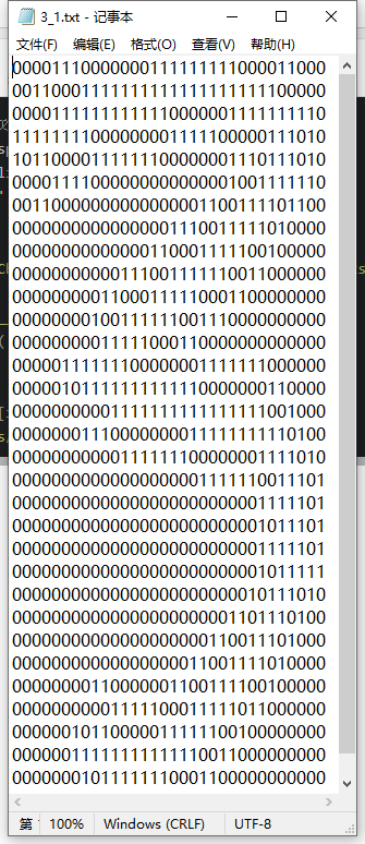
The constructed system can only recognize numbers 0 to 9. The directory trainingDigits contains about 2000 examples, and each number has about 200 samples; The directory testDigits contains about 900 test data. Although storing images in text format can not make effective use of memory space, in order to facilitate understanding, we convert images into text format. The text format of numbers is shown in the figure.

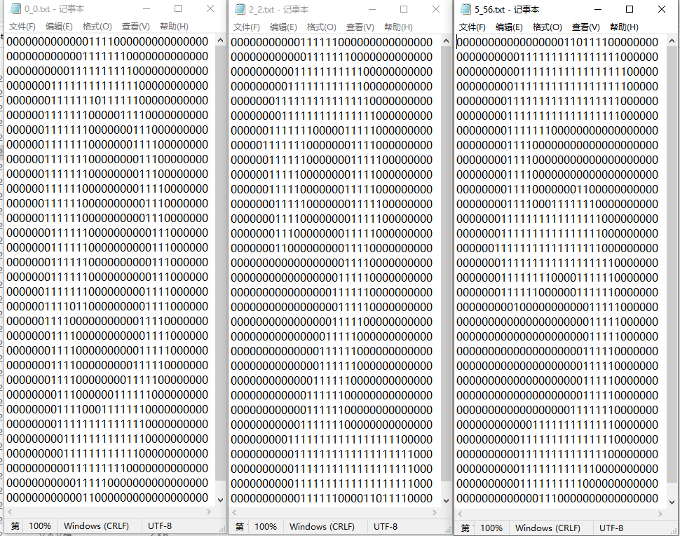
The name of the file also has special meaning. The format is: numeric value_ The sample serial number of the number.

In order to use the previous classifier, a 32 × The binary image matrix of 32 is converted to 1 × 1024 vector

'''
Parameters:
    filename - file name
Returns:
    returnVect - 1 of the binary image returned x1024 vector
'''

def img2vector(filename):
    # Create 1x1024 zero vector
    returnVect = np.zeros((1, 1024))
    # Open file
    fr = open(filename)
    # Read by line
    for i in range(32):
        # Read a row of data
        lineStr = fr.readline()
        # The first 32 elements of each row are added to returnVect in turn
        for j in range(32):
            returnVect[0, 32*i+j] = int(lineStr[j])
    # Returns the converted 1x1024 vector
    return returnVect

if __name__ == '__main__':
	testVector = img2vector('digits/testDigits/0_0.txt')
    print(testVector[0, 0:31])
    print(testVector[0, 32:63])

>>>
[0. 0. 0. 0. 0. 0. 0. 0. 0. 0. 0. 0. 0. 1. 1. 0. 0. 0. 0. 0. 0. 0. 0. 0. 0. 0. 0. 0. 0. 0. 0.]
[0. 0. 0. 0. 0. 0. 0. 0. 0. 0. 0. 0. 1. 1. 1. 1. 1. 1. 0. 0. 0. 0. 0. 0. 0. 0. 0. 0. 0. 0. 0.]

2. Test algorithm: use k-nearest neighbor algorithm to recognize handwritten digits

# Function Description: handwritten numeral classification test
def handwritingClassTest():
    # Labels for test sets
    hwLabels = []
    # Returns the file name in the trainingDigits directory
    trainingFileList = listdir('digits/trainingDigits')
    # Returns the number of files in the folder
    m = len(trainingFileList)
    # Initialize the training Mat matrix and test set
    trainingMat = np.zeros((m, 1024))
    # Resolve the category of the training set from the file name
    for i in range(m):
        # Get the name of the file
        fileNameStr = trainingFileList[i]
        # Get the number of categories
        classNumber = int(fileNameStr.split('_')[0])
        # Add the obtained categories to hwLabels
        hwLabels.append(classNumber)
        # Store 1x1024 data of each file in the trainingMat matrix
        trainingMat[i, :] = img2vector('digits/trainingDigits/%s' % (fileNameStr))
    # Returns the list of files in the testDigits directory
    testFileList = listdir('digits/testDigits')
    # Error detection count
    errorCount = 0.0
    # Number of test data
    mTest = len(testFileList)
    # Analyze the category of test set from the file and conduct classification test
    for i in range(mTest):
        fileNameStr = testFileList[i]
        classNumber = int(fileNameStr.split('_')[0])
        # The 1x1024 vector of the test set is obtained for training
        vectorUnderTest = img2vector('digits/testDigits/%s' % (fileNameStr))
        classifierResult = classify0(vectorUnderTest, trainingMat, hwLabels, 3)
        if(classifierResult != classNumber):
            print("\033[31m The returned result of classification is%d\t The real result is%d\033[0m" % (classifierResult, classNumber))
            errorCount += 1.0
        else:
            print("The returned result of classification is%d\t The real result is%d" % (classifierResult, classNumber))
    print("All wrong%d Data\n The error rate is%f%%" % (errorCount, errorCount/mTest *100))

if __name__ == '__main__':
	    handwritingClassTest()

The returned result of classification is 0	The true result is 0
 The returned result of classification is 0	The true result is 0
......
The returned result of classification is 1	The true result is 1
 The returned result of classification is 7	The true result is 1
......
The returned result of classification is 9	The true result is 9
 The returned result of classification is 5	The true result is 9
 The returned result of classification is 9	The true result is 9
 A total of 12 wrong data
 The error rate is 1.268499%

Attachment: image format conversion

Convert the picture into 32x32 array and store it in text file
The main process is to open the picture, denoise it, grayscale it, and finally set a threshold to save the binarization into a 32 * 32 array.

from PIL import Image
import matplotlib.pylab as plt
import numpy as np
from os import listdir

'''
Parameters:
    filename - file name
Returns:
    nothing
'''
# Function Description: convert the picture into a 32 * 32 pixel file, represented by 0 and 1
def picTo01(filename):
    # Open picture
    img = Image.open(filename).convert('RGBA')
    # Get the pixel value of the picture
    raw_data = img.load()
    # Gets the width and height of the picture
    width = img.size[0]
    height = img.size[1]
    # Reduce noise and convert it to black and white
    for i in range(height):
        for j in range(width):
            if raw_data[j, i][0] < 90:
                raw_data[j, i] = (0, 0, 0, 255)

    for i in range(height):
        for j in range(width):
            if raw_data[j, i][1] < 136:
                raw_data[j, i] = (0, 0, 0, 255)

    for i in range(height):
        for j in range(width):
            if raw_data[j, i][2] > 0:
                raw_data[j, i] = (255, 255, 255, 255)

    # Set to 32 * 32
    img = img.resize((32, 32), Image.LANCZOS)
    # Save
    img.save('test.png')
    # Get the pixel array as (32, 32, 4)
    array = plt.array(img)
    # Change it to 01 according to the formula
    gray_array = np.zeros((32, 32))

    for i in range(array.shape[0]):
        for j in range(array.shape[1]):
            # Calculate the gray level. If it is 255, it is white. The smaller the value, the closer it is to black
            gray = 0.299 * array[i][j][0] + 0.587 * array[i][j][1] + 0.114 * array[i][j][2]
            # Set a threshold and mark it as 0
            if gray == 255:
                gray_array[i][j] = 0
            else:
                # Otherwise, it is black and recorded as 1
                gray_array[i][j] = 1

    # Get the txt file with the corresponding name
    name01 = filename.split('.')[0]
    name01 = name01.split('/')[-1]
    name01 = name01 + '.txt'

    # Save to file
    np.savetxt('F:\\PyCharm 2021.2.1\\pythonProject\\tests\\digits\\textDigits\\' + name01, gray_array, fmt='%d', delimiter='')

if __name__ == '__main__':
    fileList = listdir('digits/imageDigits')
    m = len(fileList)
    for i in range(m):
        print(fileList[i])
        picTo01('digits/imageDigits/' + fileList[i])

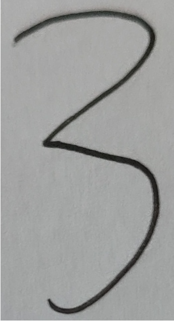
Original picture

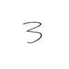
Generated 32x32 black and white picture

Generated 32x32 array text file