1, Introduction to Logistic regression

Logistic regression is a widely used classification machine learning algorithm. It fits the data into a logistic function (or logistic function), so as to predict the probability of events. To say logistic regression, we have to trace back to linear regression. We must all have a certain understanding of linear regression, that is, for the sample points existing in multidimensional space, we use the linear combination of features to fit the distribution and trajectory of the points in space. As shown in the figure below:
 

 

  Linear regression can predict continuous value results, and another common problem in real life is classification. The simplest case is the binary classification problem of yes and No. For example, the doctor needs to judge whether the patient is ill, the bank needs to judge whether a person's credit level can send him a credit card, and the e-mail inbox should automatically classify the e-mail into normal e-mail and spam, etc. In many practical cases, the classification data we need to learn is not so accurate. For example, in the above example, a data point that does not play cards according to the routine suddenly appears. The data of real-life classification problems will be more complex. At this time, it is difficult for us to complete a robust classifier with the help of linear regression threshold. Suppose there are some data points, we use a straight line to fit these points (the line is called the best fitting line), and this fitting process is called regression. The main idea of using Logistic regression for classification is to establish a regression formula for the classification boundary line according to the existing data. The word "regression" here comes from the best fitting, which means to find the best fitting parameter set. The method of training classifier is to find the best fitting parameters, and the optimization algorithm is used.
 

1. General process of Logistic regression

1) Data collection: collect data by any method.
2) Prepare data: since distance calculation is required, the data type is required to be numerical. In addition, the structured data format is the best.
3) Analyze data: analyze the data by any method.
4) Training algorithm: most of the time will be used for training. The purpose of training is to find the best classification regression coefficient.
5) Test algorithm: once the training steps are completed, the classification will be fast.
6) Using algorithm: first, we need to input some data and convert it into corresponding structured values; Then, based on the trained regression coefficients, these values can be simply regressed to determine which category they belong to; After that, we can do some other analysis work on the output categories.
 

  2. Characteristics of logistic regression

Advantages: low computational cost, easy to understand and implement.
Disadvantages: it is easy to under fit, and the classification accuracy may not be high.
Applicable data types: numerical data and nominal data.

2, Code implementation

1. logistic regression gradient rising optimization algorithm

def loadDataSet():
    dataMat = []; labelMat = []
    fr = open('testSet.txt')
    for line in fr.readlines():
        lineArr = line.strip().split()
        dataMat.append([1.0, float(lineArr[0]), float(lineArr[1])])
        labelMat.append(int(lineArr[2]))
    return dataMat,labelMat
 
def sigmoid(inX):
    return 1.0/(1+exp(-inX))
 
def gradAscent(dataMatIn, classLabels):
    dataMatrix = mat(dataMatIn)             #convert to NumPy matrix
    labelMat = mat(classLabels).transpose() #convert to NumPy matrix
    m,n = shape(dataMatrix)
    alpha = 0.001
    maxCycles = 500
    weights = ones((n,1))
    for k in range(maxCycles):              #heavy on matrix operations
        h = sigmoid(dataMatrix*weights)     #matrix mult
        error = (labelMat - h)              #vector subtraction
        weights = weights + alpha * dataMatrix.transpose()* error #matrix mult
    return weights

2. Draw the function of the best fitting line between the data set and logistic regression

def plotBestFit(weights):
    import matplotlib.pyplot as plt
    dataMat,labelMat=loadDataSet()
    dataArr = array(dataMat)
    n = shape(dataArr)[0] 
    xcord1 = []; ycord1 = []
    xcord2 = []; ycord2 = []
    for i in range(n):
        if int(labelMat[i])== 1:
            xcord1.append(dataArr[i,1]); ycord1.append(dataArr[i,2])
        else:
            xcord2.append(dataArr[i,1]); ycord2.append(dataArr[i,2])
    fig = plt.figure()
    ax = fig.add_subplot(111)
    ax.scatter(xcord1, ycord1, s=30, c='red', marker='s')
    ax.scatter(xcord2, ycord2, s=30, c='green')
    x = arange(-3.0, 3.0, 0.1)
    y = (-weights[0]-weights[1]*x)/weights[2]
    ax.plot(x, y)
    plt.xlabel('X1'); plt.ylabel('X2');
    plt.show()

3. Random gradient rise algorithm

def stocGradAscent0(dataMatrix, classLabels):
    m,n = shape(dataMatrix)
    alpha = 0.01
    weights = ones(n)   #initialize to all ones
    for i in range(m):
        h = sigmoid(sum(dataMatrix[i]*weights))
        error = classLabels[i] - h
        weights = weights + alpha * error * dataMatrix[i]
    return weights

  4. Improved random gradient rise algorithm

def stocGradAscent1(dataMatrix, classLabels, numIter=150):
    m,n = shape(dataMatrix)
    weights = ones(n)   #initialize to all ones
    for j in range(numIter):
        dataIndex = range(m)
        for i in range(m):
            alpha = 4/(1.0+j+i)+0.0001    #apha decreases with iteration, does not 
            randIndex = int(random.uniform(0,len(dataIndex)))#go to 0 because of the constant
            h = sigmoid(sum(dataMatrix[randIndex]*weights))
            error = classLabels[randIndex] - h
            weights = weights + alpha * error * dataMatrix[randIndex]
            del(dataIndex[randIndex])
    return weights

5. Test algorithm: classify with logistic regression  

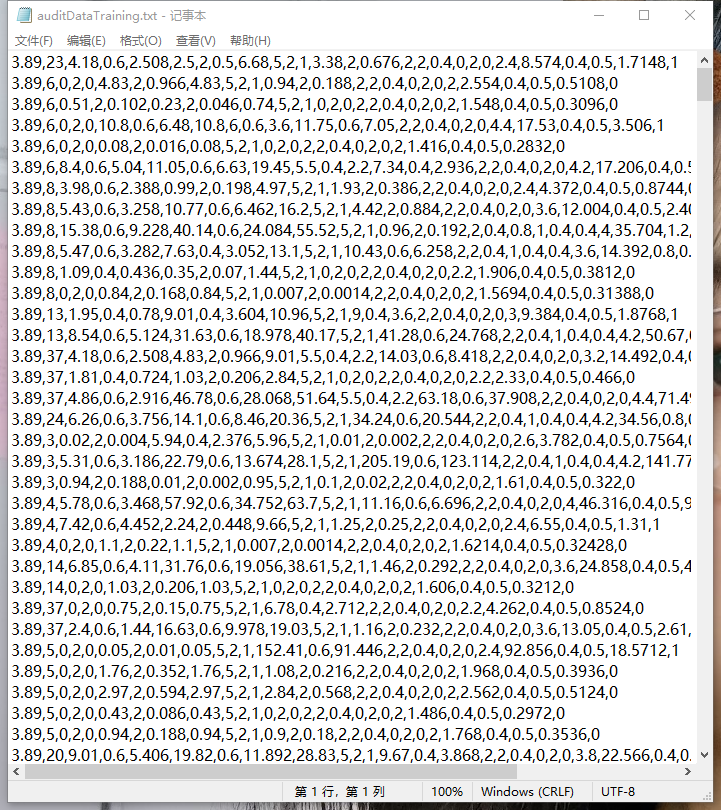
Data set used in the experiment

 

  logistic regression was used to calculate the classification error rate.

def classifyVector(inX, weights):
    prob = sigmoid(sum(inX*weights))
    if prob > 0.5: return 1.0
    else: return 0.0
 
def auditTest():
    frTrain = open('auditDataTraining.txt'); frTest = open('auditDataTest.txt')
    trainingSet = []; trainingLabels = []
    for line in frTrain.readlines():
        currLine = line.strip().split(',')
        lineArr =[]
        for i in range(26):
            lineArr.append(float(currLine[i]))
        trainingSet.append(lineArr)
        trainingLabels.append(float(currLine[26]))
    trainWeights = stocGradAscent1(array(trainingSet), trainingLabels, 1000)
    errorCount = 0; numTestVec = 0.0
    for line in frTest.readlines():
        numTestVec += 1.0
        currLine = line.strip().split(',')
        lineArr =[]
        for i in range(26):
            lineArr.append(float(currLine[i]))
        if int(classifyVector(array(lineArr), trainWeights))!= int(currLine[26]):
            errorCount += 1
    errorRate = (float(errorCount)/numTestVec)
    print "the error rate of this test is: %f" % errorRate
    return errorRate
 
def multiTest():
    numTests = 10; errorSum=0.0
    for k in range(numTests):
        errorSum += auditTest()
    print "after %d iterations the average error rate is: %f" % (numTests, errorSum/float(numTests))

  After running multiTest()

  The average error rate is very low. It seems that there are few missing data in this dataset.