%matplotlib inline
import matplotlib.pyplot as plt
import numpy as np
1. PCA introduction
1.1 concept
Thought:

dots = np.array([[1, 1.5], [2, 1.5], [3, 3.6], [4, 3.2], [5, 5.5]])

def cross_point(x0, y0):
    """
    1. line1: y = x
    2. line2: y = -x + b => x = b/2
    3. [x0, y0] is in line2 => b = x0 + y0

    => x1 = b/2 = (x0 + y0) / 2
    => y1 = x1
    """
    x1 = (x0 + y0) / 2
    return x1, x1


plt.figure(figsize=(8, 6), dpi=144)
plt.title('2-dimension to 1-dimension')

plt.xlim(0, 8)
plt.ylim(0, 6)
ax = plt.gca()                                  # gca represents the current coordinate axis, that is, 'get current axis'
ax.spines['right'].set_color('none')            # Hide axes
ax.spines['top'].set_color('none')

plt.scatter(dots[:, 0], dots[:, 1], marker='s', c='b')
plt.plot([0.5, 6], [0.5, 6], '-r')
for d in dots:
    x1, y1 = cross_point(d[0], d[1])
    plt.plot([d[0], x1], [d[1], y1], '--b')
    plt.scatter(x1, y1, marker='o', c='r')
plt.annotate(r'projection point',
             xy=(x1, y1), xycoords='data',
             xytext=(x1 + 0.5, y1 - 0.5), fontsize=10,
             arrowprops=dict(arrowstyle="->", connectionstyle="arc3,rad=.2"))
plt.annotate(r'vector $u^{(1)}$',
             xy=(4.5, 4.5), xycoords='data',
             xytext=(5, 4), fontsize=10,
             arrowprops=dict(arrowstyle="->", connectionstyle="arc3,rad=.2"))
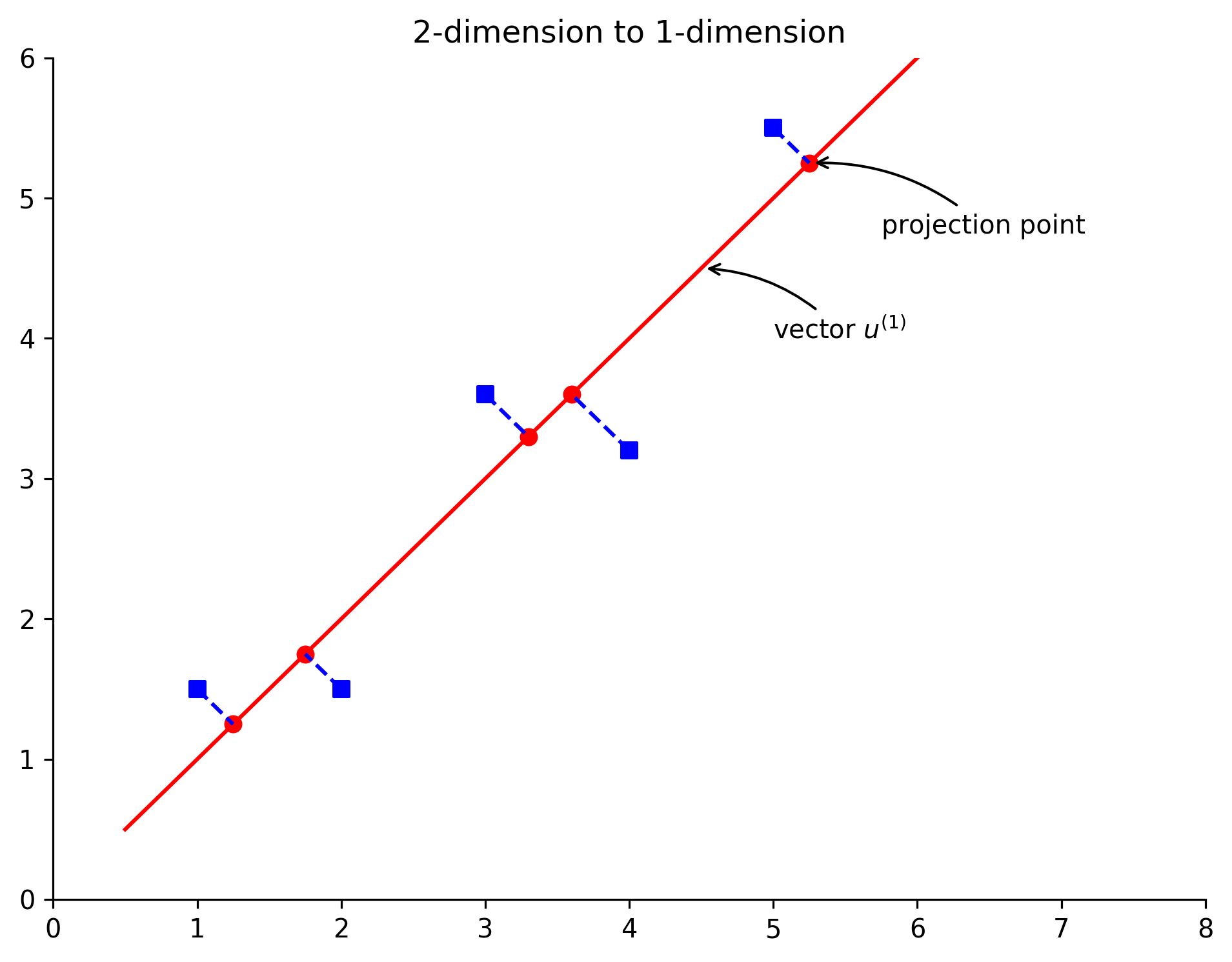
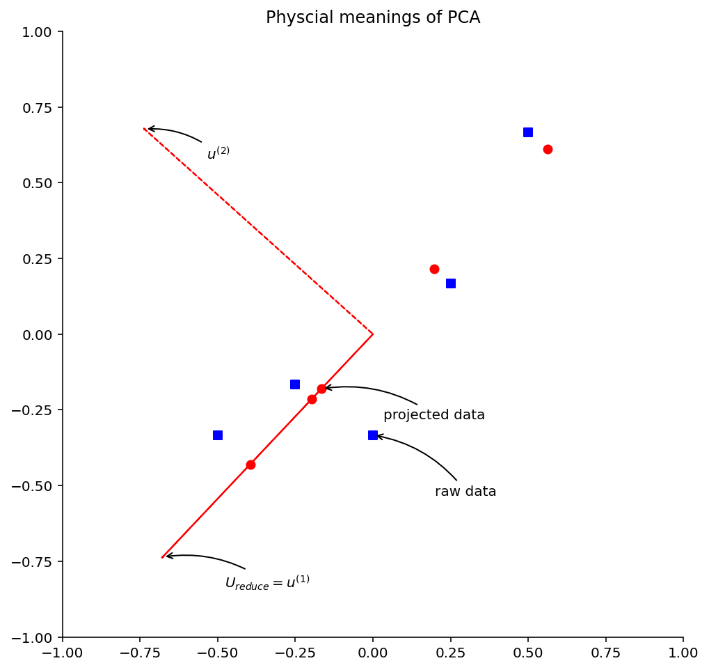
The square point in the figure is the data after preprocessing (normalization and scaling) of the original data, and the circular point is the data recovered from one dimension to two dimensions. At the same time, we draw the principal component eigenvectors U1 and U2. According to the above figure, several interesting conclusions are introduced: first, the circular point is actually the projection of the square point on the line where the vectors U1 and U2 are located. The so-called PCA data recovery is not real recovery, but the coordinates after dimension reduction are transformed into the coordinates in the original coordinate system. For our example, we just convert the coordinates in the one-dimensional coordinate system determined by vectors U1 and U2 into the coordinates in the original two-dimensional coordinate system. Secondly, the principal component eigenvectors U1 and U2 are perpendicular to each other. Thirdly, the distance between square points and circular points is the error of PCA data after dimensionality reduction.
1.2 schematic diagram of dimension reduction and recovery
plt.figure(figsize=(8, 8), dpi=144)

plt.title('Physcial meanings of PCA')

ymin = xmin = -1
ymax = xmax = 1
plt.xlim(xmin, xmax)
plt.ylim(ymin, ymax)
ax = plt.gca()                                  # gca represents the current coordinate axis, that is, 'get current axis'
ax.spines['right'].set_color('none')            # Hide axes
ax.spines['top'].set_color('none')

plt.scatter(norm[:, 0], norm[:, 1], marker='s', c='b')
plt.scatter(Z[:, 0], Z[:, 1], marker='o', c='r')
plt.arrow(0, 0, U[0][0], U[1][0], color='r', linestyle='-')
plt.arrow(0, 0, U[0][1], U[1][1], color='r', linestyle='--')
plt.annotate(r'$U_{reduce} = u^{(1)}$',
             xy=(U[0][0], U[1][0]), xycoords='data',
             xytext=(U_reduce[0][0] + 0.2, U_reduce[1][0] - 0.1), fontsize=10,
             arrowprops=dict(arrowstyle="->", connectionstyle="arc3,rad=.2"))
plt.annotate(r'$u^{(2)}$',
             xy=(U[0][1], U[1][1]), xycoords='data',
             xytext=(U[0][1] + 0.2, U[1][1] - 0.1), fontsize=10,
             arrowprops=dict(arrowstyle="->", connectionstyle="arc3,rad=.2"))
plt.annotate(r'raw data',
             xy=(norm[0][0], norm[0][1]), xycoords='data',
             xytext=(norm[0][0] + 0.2, norm[0][1] - 0.2), fontsize=10,
             arrowprops=dict(arrowstyle="->", connectionstyle="arc3,rad=.2"))
plt.annotate(r'projected data',
             xy=(Z[0][0], Z[0][1]), xycoords='data',
             xytext=(Z[0][0] + 0.2, Z[0][1] - 0.1), fontsize=10,
             arrowprops=dict(arrowstyle="->", connectionstyle="arc3,rad=.2"))
Text(0.03390904029252009, -0.28050757997562326, 'projected data')
2. PCA algorithm simulation
2.1 Numpy implementation
A = np.array([[3, 2000],
              [2, 3000],
              [4, 5000],
              [5, 8000],
              [1, 2000]], dtype='float')

# data normalization
mean = np.mean(A, axis=0)
norm = A - mean
# Data scaling
scope = np.max(norm, axis=0) - np.min(norm, axis=0)
norm = norm / scope
norm
array([[ 0.        , -0.33333333],
       [-0.25      , -0.16666667],
       [ 0.25      ,  0.16666667],
       [ 0.5       ,  0.66666667],
       [-0.5       , -0.33333333]])
U, S, V = np.linalg.svd(np.dot(norm.T, norm))
U
array([[-0.67710949, -0.73588229],
       [-0.73588229,  0.67710949]])
U_reduce = U[:, 0].reshape(2,1)
U_reduce
array([[-0.67710949],
       [-0.73588229]])
R = np.dot(norm, U_reduce)
R
array([[ 0.2452941 ],
       [ 0.29192442],
       [-0.29192442],
       [-0.82914294],
       [ 0.58384884]])
Z = np.dot(R, U_reduce.T)
Z
array([[-0.16609096, -0.18050758],
       [-0.19766479, -0.21482201],
       [ 0.19766479,  0.21482201],
       [ 0.56142055,  0.6101516 ],
       [-0.39532959, -0.42964402]])
np.multiply(Z, scope) + mean
array([[2.33563616e+00, 2.91695452e+03],
       [2.20934082e+00, 2.71106794e+03],
       [3.79065918e+00, 5.28893206e+03],
       [5.24568220e+00, 7.66090960e+03],
       [1.41868164e+00, 1.42213588e+03]])
2.2 implementation of sklearn package
from sklearn.decomposition import PCA
from sklearn.pipeline import Pipeline
from sklearn.preprocessing import MinMaxScaler

def std_PCA(**argv):
    # MinMaxScaler preprocesses the data
    scaler = MinMaxScaler()
    # PCA algorithm
    pca = PCA(**argv)
    pipeline = Pipeline([('scaler', scaler),
                         ('pca', pca)])
    return pipeline

pca = std_PCA(n_components=1)
R2 = pca.fit_transform(A)
R2
array([[-0.2452941 ],
       [-0.29192442],
       [ 0.29192442],
       [ 0.82914294],
       [-0.58384884]])
pca.inverse_transform(R2)
array([[2.33563616e+00, 2.91695452e+03],
       [2.20934082e+00, 2.71106794e+03],
       [3.79065918e+00, 5.28893206e+03],
       [5.24568220e+00, 7.66090960e+03],
       [1.41868164e+00, 1.42213588e+03]])
3. Example: face dimensionality reduction by pca
%matplotlib inline
import matplotlib.pyplot as plt
import numpy as np
from sklearn.datasets import fetch_olivetti_faces

# fetch_ olivetti_ The faces function can help us intercept the middle part, leaving only facial features
faces = fetch_olivetti_faces(data_home='datasets/')

X = faces.data
y = faces.target
image = faces.images
print("data:{}, label:{}, image:{}".format(X.shape, y.shape, image.shape))
data:(400, 4096), label:(400,), image:(400, 64, 64)
View some images
target_names = np.array(["c%d" % i for i in np.unique(y)])
target_names
array(['c0', 'c1', 'c2', 'c3', 'c4', 'c5', 'c6', 'c7', 'c8', 'c9', 'c10',
       'c11', 'c12', 'c13', 'c14', 'c15', 'c16', 'c17', 'c18', 'c19',
       'c20', 'c21', 'c22', 'c23', 'c24', 'c25', 'c26', 'c27', 'c28',
       'c29', 'c30', 'c31', 'c32', 'c33', 'c34', 'c35', 'c36', 'c37',
       'c38', 'c39'], dtype='<U3')
plt.figure(figsize=(12, 11), dpi=100)
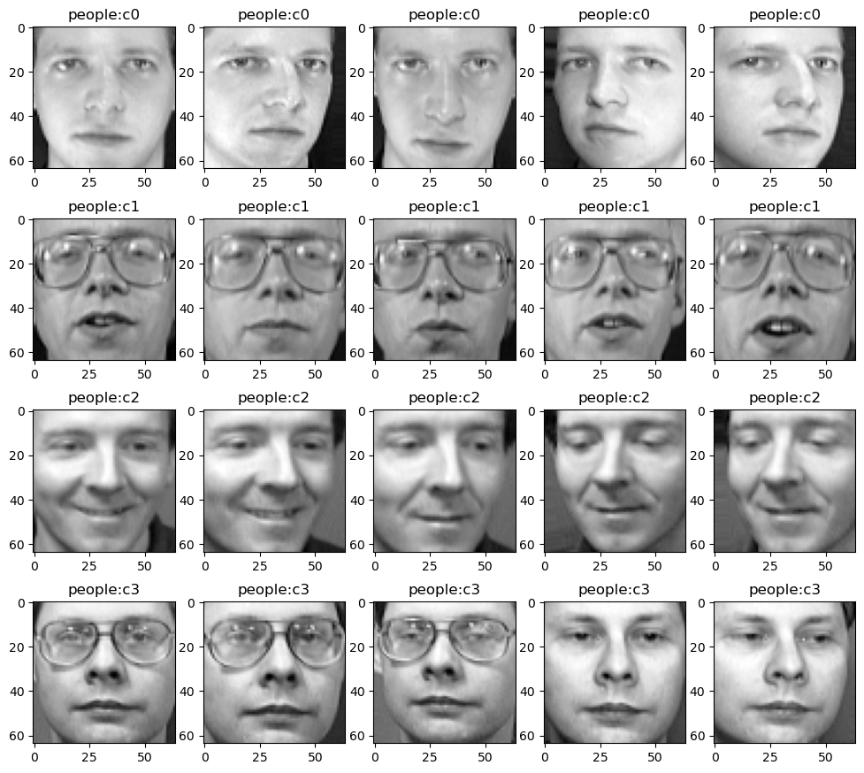
# Five images of two people are displayed here
shownum = 40
# Extract the names of the first k people
title = target_names[:int(shownum/10)]
j = 1
# Each person's 10 images are displayed in front of the theme song
for i in range(shownum):
if i%10 < 5:
plt.subplot(int(shownum/10),5,j)
plt.title("people:"+title[int(i/10)])
plt.imshow(image[i],cmap=plt.cm.gray)
j+=1
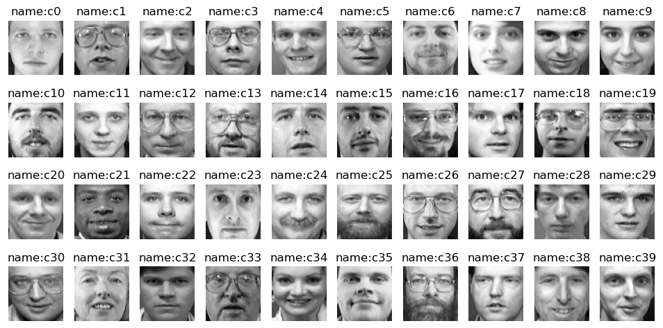
The first image of all 40 people was extracted and displayed
subimage = None

for i in range(len(image)):
    if i%10 == 0:
        if subimage is not None:
#             print("subimage.shape:{},image[i].shape:{}",subimage.shape, image[i].shape)
            subimage = np.concatenate((subimage, image[i].reshape(1,64,64)), axis=0)
        else:
            subimage = image[i].reshape(1,64,64)

plt.figure(figsize=(12,6), dpi=100)

for i in range(subimage.shape[0]):
    plt.subplot(int(subimage.shape[0]/10), 10, i+1)
    plt.imshow(subimage[i], cmap=plt.cm.gray)
    plt.title("name:"+target_names[i])
    plt.axis('off')
Partition dataset
from sklearn.model_selection import train_test_split

X_train, X_test, y_train, y_test = train_test_split(
    X, y, test_size=0.2, random_state=4)

X_train.shape, X_test.shape, y_train.shape, y_test.shape
((320, 4096), (80, 4096), (320,), (80,))
Using svm to realize face recognition
from sklearn.svm import SVC

# Specifies the class of SVC_ The weight parameter enables the SVC model to adjust the weight evenly according to the number of training samples
clf = SVC(class_weight='balanced')
# train
clf.fit(X_train, y_train)
# Calculate score
trainscore = clf.score(X_train,y_train)
testscore = clf.score(X_test,y_test)
print("trainscore:{},testscore:{}".format(trainscore, testscore))
# forecast
y_pred = clf.predict(X_test)
trainscore:1.0,testscore:0.975
Display test set images
# plt.figure(figsize=(12,6), dpi=100)
plt.subplot(1,1,1)
plt.imshow(X_test[1].reshape(64,64), cmap=plt.cm.gray)
<matplotlib.image.AxesImage at 0x21fb6d83688>
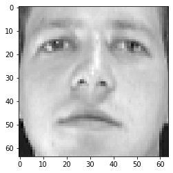
The prediction is correct. It can be found that the prediction effect of svm is very good
y_test[1] == y_pred[1]
True
The PCA model is explained_ variance_ The ratio variable can obtain the data restoration rate after PCA processing
from sklearn.decomposition import PCA

pca = PCA(n_components=140)
X_pca = pca.fit_transform(X)
np.sum(pca.explained_variance_ratio_)
0.9585573
Now 4096 features are used. Now PCA is used to reduce the dimension of the features, and then view the changes of the image;
from sklearn.decomposition import PCA

# Original drawing display
plt.figure(figsize=(12,8), dpi=100)
subimage = faces.images[:5]
for i in range(5):
    plt.subplot(1, 5, i+1)
    plt.imshow(subimage[i], cmap=plt.cm.gray)
    plt.axis('off')

# Image display after dimensionality reduction
k = [140, 75, 37, 19, 8]
plt.figure(figsize=(12,12), dpi=100)

for index in range(len(k)):
    pca = PCA(n_components=k[index])

    # Dimensionality reduction
    X_pca = pca.fit_transform(X)
    # The dimension is upgraded again, and there is loss in the intermediate process
    X_invert_pca = pca.inverse_transform(X_pca)
    image = X_invert_pca.reshape(-1,64,64)
    subimage = image[:5]

    for i in range(len(k)):
        plt.subplot(len(k), 5, (i+1)+len(k)*index)
        plt.imshow(subimage[i], cmap=plt.cm.gray)
    #     plt.title("name:"+target_names[i])
        plt.axis('off')

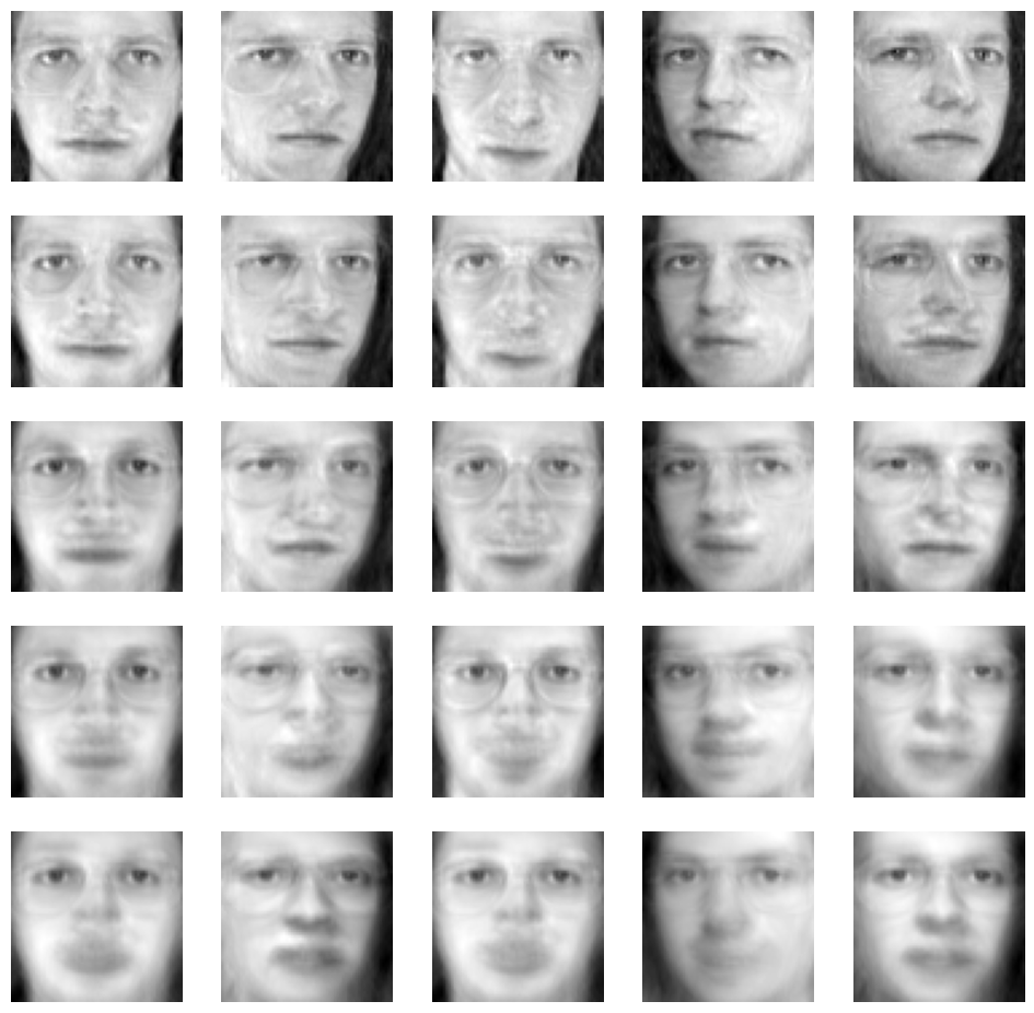
It can be seen that the face is gradually blurred after dimension reduction. From 4096 feature dimension to 140 dimension, most of the features of the face can be maintained
https://zhuanlan.zhihu.com/p/271969151 About fit(), transform(), fit_ The difference between transform() is introduced in this blog
You must use fit first_ Transform (traindata), and then transform(testData). If you directly transform(testData), the program will report an error
If fit_ After transfrom (traindata), use fit_transform(testData) instead of transform(testData) can also be normalized, but the two results are not under the same "standard" and have obvious differences. That is, we need to process the test set with the normalization process of processing the training set to ensure the same data processing.
from sklearn.svm import SVC

# Set multi drop dimensions
pca = PCA(n_components=140)

# Firstly, the training set pair is used for training and normalization
X_train_pca = pca.fit_transform(X_train)
# Then, the same parameters of the training set are normalized
X_test_pca = pca.transform(X_test)

# Specifies the class of SVC_ The weight parameter enables the SVC model to adjust the weight evenly according to the number of training samples
clf = SVC(class_weight='balanced')
# svm is trained with normalized data
clf.fit(X_train_pca, y_train)

# Calculate score
trainscore = clf.score(X_train_pca,y_train)
testscore = clf.score(X_test_pca,y_test)
print("trainscore:{},testscore:{}".format(trainscore, testscore))
trainscore:1.0,testscore:0.975
Use GridSearchCV to further filter
from sklearn.model_selection import GridSearchCV

# print("Searching the best parameters for SVC ...")
param_grid = {'C': [1, 5, 10, 50, 100],
              'gamma': [0.0001, 0.0005, 0.001, 0.005, 0.01]}
clf = GridSearchCV(SVC(kernel='rbf', class_weight='balanced'), param_grid, verbose=2, n_jobs=4)
clf = clf.fit(X_train_pca, y_train)
print("Best parameters found by grid search:",clf.best_params_)

# Calculate score
trainscore = clf.score(X_train_pca,y_train)
testscore = clf.score(X_test_pca,y_test)
print("trainscore:{},testscore:{}".format(trainscore, testscore))
Fitting 5 folds for each of 25 candidates, totalling 125 fits
Best parameters found by grid search: {'C': 5, 'gamma': 0.005}
trainscore:1.0,testscore:0.9625
It can be seen that the effect is very good
import pandas as pd

result = pd.DataFrame()
result['pred'] = y_pred
result['true'] = y_test
result['compares'] = y_pred==y_test
result.head(10)
| pred | true | compares | |
|---|---|---|---|
| 0 | 18 | 18 | True |
| 1 | 0 | 0 | True |
| 2 | 6 | 6 | True |
| 3 | 31 | 31 | True |
| 4 | 10 | 10 | True |
| 5 | 27 | 27 | True |
| 6 | 36 | 36 | True |
| 7 | 32 | 32 | True |
| 8 | 29 | 29 | True |
| 9 | 33 | 33 | True |