Tip: here is a hard Ken 📕 If Xiaobai makes a mistake, change it. Don't spray it:)

preface

The sky can be mended, the sea can be filled, the mountains can be moved, the sun and the moon are past, and can not be pursued again.

Decision Tree is based on tree structure to make decisions. (classification, regression)
A decision tree contains a root node, several internal nodes and several leaf nodes.
The ultimate goal is to divide the sample more and more pure.
"Bole Xiangma" good allusion!!! (from) Decision tree classification algorithm (if else principle))

tips: it's a long way to go. I'll look up and down

1, Basic algorithm of decision tree learning

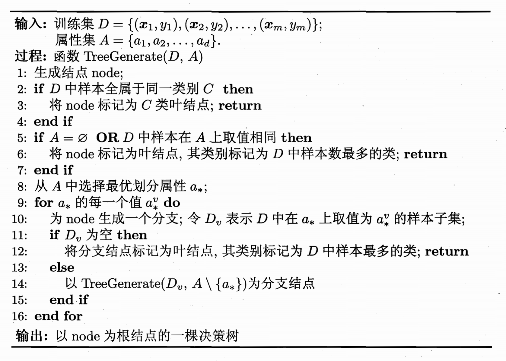
The purpose of decision tree learning is to generate a decision tree with strong generalization ability, i.e. strong ability to deal with unseen examples, and follow the "divide and conquer" strategy. Its generation is a recursive process. The following figure shows the basic algorithm process of decision tree learning in machine learning (please experience ~).

1. Information Entropy

The key of decision tree learning is how to select the optimal partition attribute. In the division process, the samples contained in the branch nodes of the decision tree belong to the same category as much as possible, and the "purity" of the nodes is higher and higher.

Information entropy is the most commonly used index to measure the purity of sample set.
Assume current sample set D D Section in D k k The proportion of class k samples is p k   ( k = 1 , 2 , . . . , ∣ y ∣ ) p_k \ (k=1,2,...,|y|) pk (k=1,2,..., ∣ y ∣), then D D The information entropy of D is defined as
E n t ( D ) = − ∑ k = 1 ∣ y ∣ p k   l o g 2   p k Ent(D)=-\sum_{k=1}^{|y|}p_k \ log_2\ p_k Ent(D)=−k=1∑∣y∣​pk​ log2​ pk​
E n t ( D ) Ent(D) The smaller the value of Ent(D), the D D The higher the purity of D.

2. Information gain - ID3 decision tree

Assumed discrete attribute a a a yes V V V possible values { a 1 , a 2 , . . . , a V } \lbrace a^1,a^2,...,a^V \rbrace {a1,a2,...,aV}, if used a a a to the sample set D D D will be generated V V V branch nodes, where v v v branch nodes contain D D All attributes in D a a The value on a is a v a^v The sample of av is D v D^v Dv.

Give weight to branch nodes ∣ D v ∣ ∣ D ∣ \frac{|D^v|} {|D|} ∣ D ∣ ∣ Dv ∣, the greater the number of samples, the greater the impact of branch nodes and the greater the information gain. Use attribute a to the sample set D D D the greater the purity improvement obtained by dividing.
G a i n ( D , a ) = E n t ( D ) − ∑ v = 1 V ∣ D v ∣ ∣ D ∣ E n t ( D v ) Gain(D,a)=Ent(D)-\sum_{v=1}^{V} \frac {|D^v|} {|D|}Ent(D^v) Gain(D,a)=Ent(D)−v=1∑V​∣D∣∣Dv∣​Ent(Dv)

ID3 (iterative dichotomizer) decision tree learning algorithm uses information gain criterion to select partition attributes.
The information gain criterion has a preference for attributes with a large number of values.
Select the optimal partition attribute from attribute set A a ∗ = a r g   m a x   a ∈ A G a i n ( D , a ) a_*=\underset{a \in A}{arg\ max\ } Gain(D,a) a∗​=a∈Aarg max ​Gain(D,a).

3. Gain Ratio - C4.5 decision tree

C4. The decision tree algorithm does not directly use the information gain, but uses the gain rate to select the optimal partition attribute.
The gain rate criterion has a preference for attributes with a small number of values.
G a i n _ r a t i o ( D , a ) = G a i n ( D , a ) I V ( a ) Gain\_ratio(D,a)= \frac {Gain(D,a)} {IV(a)} Gain_ratio(D,a)=IV(a)Gain(D,a)​
Among them, I V ( a ) = − ∑ v = 1 V ∣ D v ∣ ∣ D ∣ l o g 2 ∣ D v ∣ ∣ D ∣ IV(a)=-\sum_{v=1}^{V} \frac {|D^v|} {|D|}log_2 \frac {|D^v|} {|D|} IV(a)=−v=1∑V​∣D∣∣Dv∣​log2​∣D∣∣Dv∣​
Called the Intrinsic Value of property A. The more possible values of property a, the I V ( a ) IV(a) The value of IV(a) is usually larger.

C4. The decision tree does not completely use "gain rate" instead of "information gain", but uses a heuristic method: first select the attribute with higher information gain than the average level, and then select the attribute with the highest gain rate.

4. Gini Index - CART decision tree

CART (Classification and Regression Tree) decision tree uses Gini index to select partition attributes.
data set D D The purity of D, measured by Gini value, is:
G i n i ( D ) = ∑ k = 1 ∣ y ∣ ∑ k ′ ≠ k p k p k ′ = 1 − ∑ k = 1 ∣ y ∣ p k 2 Gini(D)=\sum_{k=1}^{|y|} \sum_{k'\not= k} p_kp_k'=1-\sum_{k=1}^{|y|}p_k^2 Gini(D)=k=1∑∣y∣​k′​=k∑​pk​pk′​=1−k=1∑∣y∣​pk2​
G i n i ( D ) Gini(D) The smaller the value of Gini(D), the D D The higher the purity of D.

The Gini index of attribute a is defined as:
G i n i _ i n d e x ( D , a ) = ∑ v = 1 V ∣ D v ∣ ∣ D ∣ G i n i ( D ) Gini\_index(D,a)= \sum_{v=1}^{V} \frac {|D^v|} {|D|} Gini(D) Gini_index(D,a)=v=1∑V​∣D∣∣Dv∣​Gini(D)
Select the attribute with the smallest Gini index from attribute set A as the optimal partition attribute a ∗ = a r g   m i n   a ∈ A G i n i _ i n d e x ( D , a ) a_*=\underset{a \in A}{arg\ min\ } Gini\_index(D,a) a∗​=a∈Aarg min ​Gini_index(D,a).

5. Pruning treatment (pruning)

Pruning is the main way for decision tree algorithm to deal with "over fitting", that is, actively removing some branches to reduce the risk of over fitting.

Friends can fill in the "Occam razor guidelines" by themselves.
Take some pictures from the book of machine learning and understand:

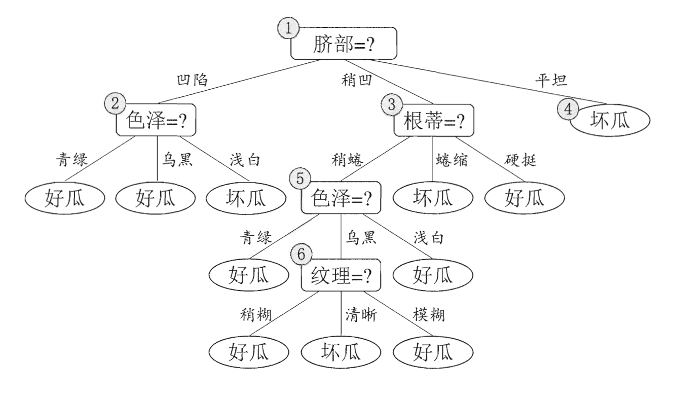
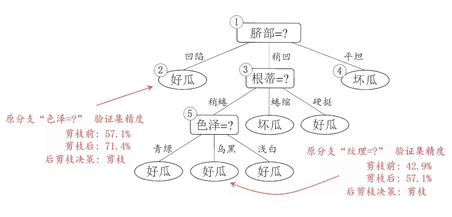
[watermelon data set] non pruned decision tree flow chart, select the attribute "navel" to divide the training set and judge the quality of watermelon.

There are two basic strategies for decision tree pruning:

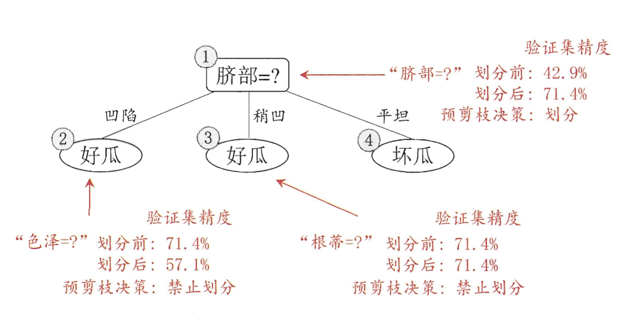
(1) Pre pruning

Pre pruning means that in the process of decision tree generation, each node is estimated before division. If the division of the current node can not improve the generalization performance of the decision tree, the division is stopped and the current node is marked as a leaf node.

(2) Post pruning

Post pruning refers to generating a complete decision tree from the training set, and then investigating the non leaf nodes from bottom to top. If replacing the subtree corresponding to the node with leaf nodes can improve the generalization performance of the decision tree, the subtree will be replaced with leaf nodes.

Post pruning decision tree often retains more branches than pre pruning decision tree. Generally, post pruning decision tree has less risk of under fitting, and its generalization ability is often better than pre pruning decision tree. However, the training time of post pruning is longer than that of non pruning and pre pruning.

2, Classification and prediction of iris data set using decision tree

Decision tree classifier in sklearn

class sklearn.tree.DecisionTreeClassifier(*, criterion='gini', splitter='best', max_depth=None, min_samples_split=2, min_samples_leaf=1, min_weight_fraction_leaf=0.0, max_features=None, random_state=None, max_leaf_nodes=None, min_impurity_decrease=0.0, class_weight=None, ccp_alpha=0.0)

• criterion: gini or entropy, the former is gini index and the latter is information entropy;
• max_depth: int or None, optional (default=None) sets the maximum depth of the decision tree in the decision random forest. The greater the depth, the easier it is to over fit. The recommended tree depth is between 5-20;
• max_features: None (all), log2, sqrt and N are generally used when the features are less than 50;
• max_leaf_nodes: over fitting can be prevented by limiting the maximum number of leaf nodes. The default is "None", that is, the maximum number of leaf nodes is not limited.

Dataset partitioning api

sklearn.model_selection.train_test_split(arrays, *options)

• Parameters:
  Eigenvalues of x dataset
  Label value of y dataset
  test_size the size of the test set, usually float
  random_state random number seeds. Different seeds will cause different random sampling results. The same seed sampling results are the same.
• return
  x_train, x_test, y_train, y_test

The code is as follows (example):

# pandas is used to process and analyze data
import pandas as pd
import numpy as np
# Import iris dataset
from sklearn.datasets import load_iris
# Import decision tree classifier
from sklearn.tree import DecisionTreeClassifier
# # Method of importing split dataset
from sklearn.model_selection import train_test_split
# import relevant packages
from sklearn import tree
from sklearn.tree import export_text
# import matplotlib; matplotlib.use('TkAgg')
import matplotlib.pyplot as plt

# Classification and prediction of iris data set using decision tree
# Dataset Field Description:
# Eigenvalues (4): sepal length, sepal width, petal length, petal width
# Target value (3): target (category, 0 is' setosa 'mountain iris, 1 is' versicolor' color changing iris, and 2 is' Virginia 'Virginia iris)

# load in the data
data = load_iris()
# convert to a dataframe
df = pd.DataFrame(data.data, columns = data.feature_names)
# create the species column
df['Species'] = data.target

# replace this with the actual names
target = np.unique(data.target)  # For a one-dimensional array or list, the unique function removes the duplicate elements and returns a new tuple or list without duplicate elements from large to small
target_names = np.unique(data.target_names)
targets = dict(zip(target, target_names))
df['Species'] = df['Species'].replace(targets)

# extract features and target variables
x = df.drop(columns="Species")
y = df["Species"]
# save the feature name and target variables
feature_names = x.columns
labels = y.unique()  # Remove duplicate elements

# Split training set and test set
# Eigenvalues of x dataset
# Label value of y dataset
# Eigenvalue X of training set_ Eigenvalue X of train test set_ Test (test_x) target value y of training set_ Target value y of train test set_ test(test_lab)
# random_state random number seeds. Different seeds will cause different random sampling results. The same seed sampling results are the same.
X_train, test_x, y_train, test_lab = train_test_split(x,y,
                                                 test_size = 0.4,
                                                 random_state = 42)
# Create a decision tree classifier (the maximum depth of the tree is 3)
model = DecisionTreeClassifier(max_depth =3, random_state = 42)  # Initialization model
model.fit(X_train, y_train)  # Training model
print(model.score(test_x,test_lab))  # Evaluation model score
# Calculate the importance of each feature
print(model.feature_importances_)

# Visual feature attribute results
r = export_text(model, feature_names=data['feature_names'])
print(r)

# plt the figure, setting a black background
plt.figure(figsize=(30,10), facecolor ='g')  # facecolor sets the background color

# create the tree plot decision tree drawing module to realize the visualization of decision tree
a = tree.plot_tree(model,
                   # use the feature names stored
                   feature_names = feature_names,
                   # use the class names stored
                   class_names = labels,
                   # label='all',
                   rounded = True,
                   filled = True,
                   fontsize=14,
                   )
# show the plot
# plt.legend(loc='lower right', borderpad=0, handletextpad=0)
plt.savefig("save.png", dpi=300, bbox_inches="tight")
# plt.tight_layout()
plt.show()

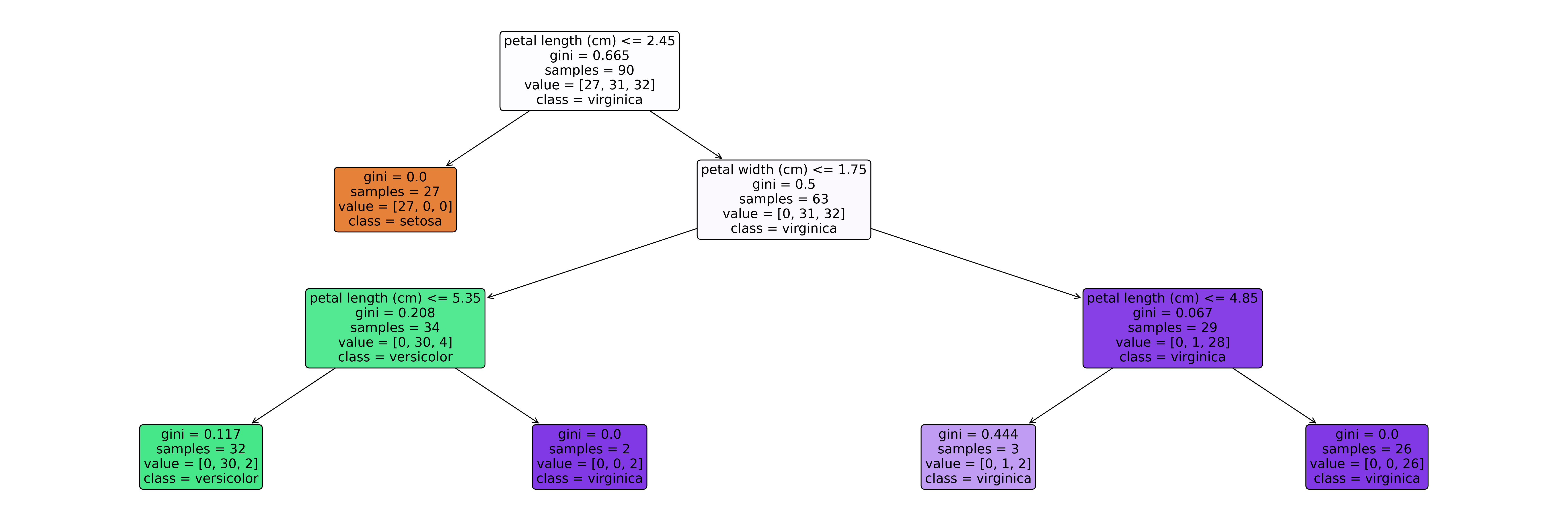
Output results:

0.9833333333333333
[0.         0.         0.58908421 0.41091579]
|--- petal length (cm) <= 2.45
|   |--- class: setosa
|--- petal length (cm) >  2.45
|   |--- petal width (cm) <= 1.75
|   |   |--- petal length (cm) <= 5.35
|   |   |   |--- class: versicolor
|   |   |--- petal length (cm) >  5.35
|   |   |   |--- class: virginica
|   |--- petal width (cm) >  1.75
|   |   |--- petal length (cm) <= 4.85
|   |   |   |--- class: virginica
|   |   |--- petal length (cm) >  4.85
|   |   |   |--- class: virginica

summary

Tip: here is a summary of the article:
For example, the above is what we want to talk about today. This paper only briefly introduces the use of pandas, which provides a large number of functions and methods that enable us to process data quickly and conveniently.