catalogue
2.1 random forest classifier function and its parameters
2.2 construction of random forest
2.3 comparison of random forest and decision tree under cross validation
2.4 drawing n_ Learning curve of estimators
3.1 random forest classifier function and its parameters
3.2 filling missing values with random forest regression
4 basic idea of machine learning parameter adjustment
1 integrated learning
Ensemble learning completes the learning task by building and combining multiple learners. It is not a single machine learning algorithm, but by building multiple models on the data to integrate the modeling results of all models. It can be used to model marketing simulation, count customer sources, retention and loss, and predict the risk of disease and the susceptibility of patients.
The integration algorithm will consider the modeling results of multiple evaluators and summarize them to obtain a comprehensive result, so as to obtain better regression or classification performance than a single model.
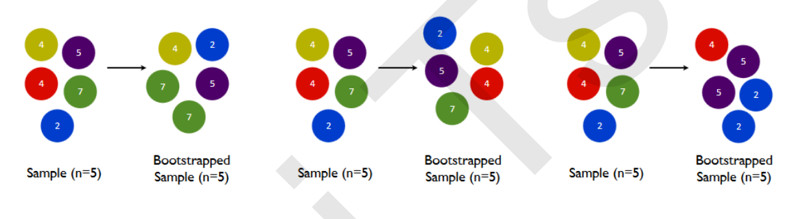
The model integrated by multiple models is called an integrated estimator, and each model constituting the integrated estimator is called a base estimator. Generally speaking, there are three kinds of integration algorithms: Bagging, Boosting and stacking.

To achieve good integration, individual learners should be "good but different", that is, individual learners should not only have certain accuracy, but also have differences between learners.
2 random forest classifier
2.1 random forest classifier function and its parameters
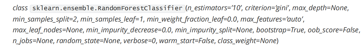
Many parameters of random forest classifier are consistent with those of decision tree. The parameters of the control base evaluator are as follows.
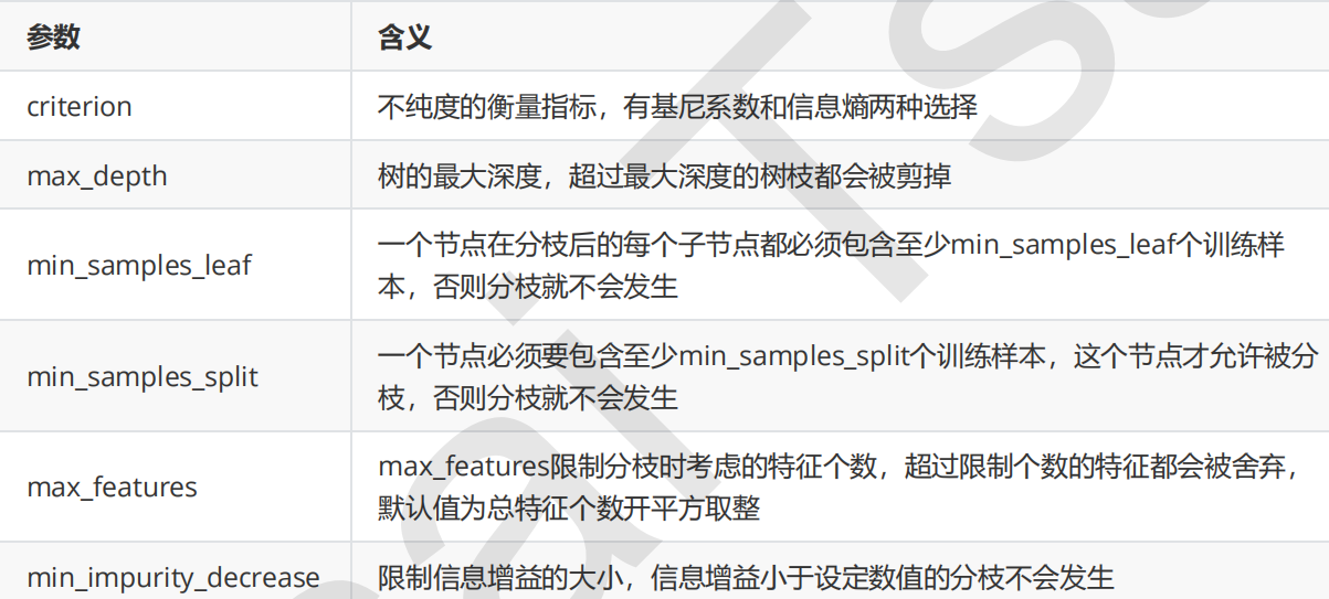
Other relevant parameters:

2.2 construction of random forest
On the red wine dataset, the effect of random forest is better than that of decision tree.
from sklearn.ensemble import RandomForestClassifier
from sklearn.tree import DecisionTreeClassifier
from sklearn.model_selection import train_test_split
from sklearn.datasets import load_wine
wine=load_wine()
Xtrain,Xtest,Ytrain,Ytest=train_test_split(wine.data,wine.target,test_size=0.3)
#instantiation
clf=DecisionTreeClassifier()
rfc=RandomForestClassifier()
clf=clf.fit(Xtrain,Ytrain)
rfc.fit(Xtrain,Ytrain)
score_c=clf.score(Xtest,Ytest)
score_r=rfc.score(Xtest,Ytest)
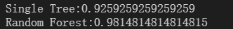
print("Single Tree:{}".format(score_c))
print("Random Forest:{}".format(score_r))
2.3 comparison of random forest and decision tree under cross validation
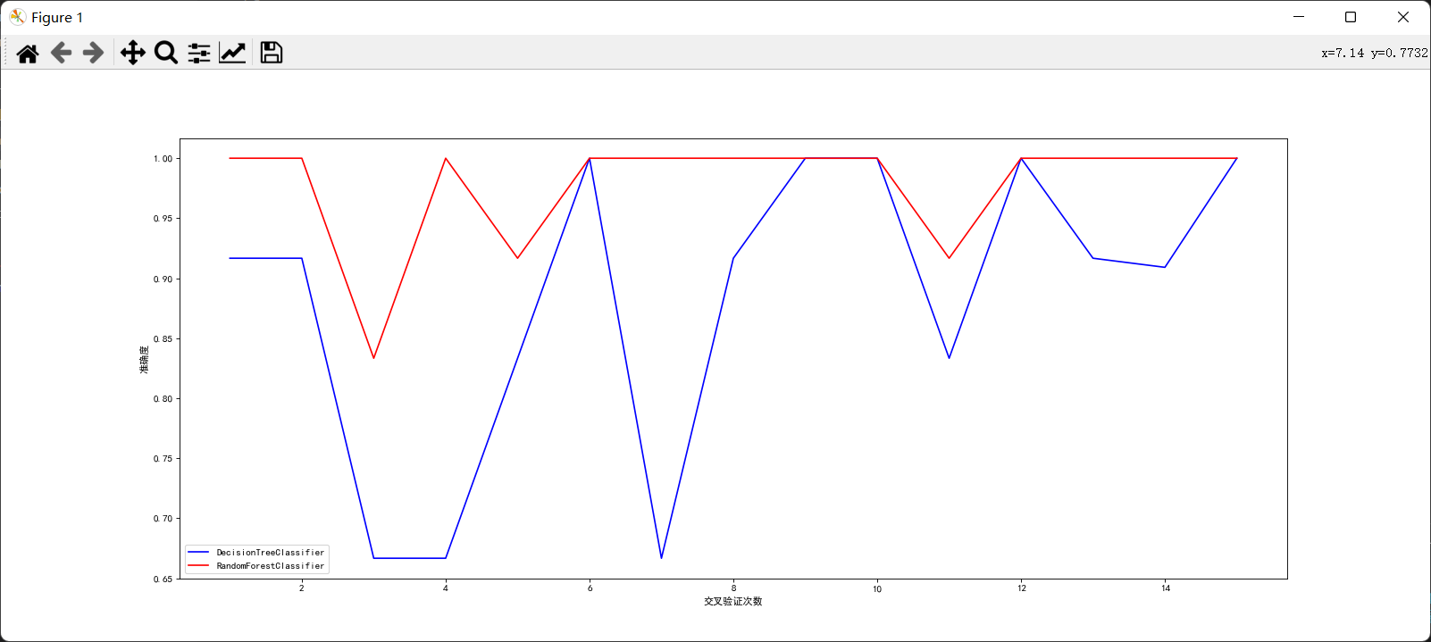
Through comparison, it can be found that the effect of random forest is indeed better than decision tree. Only in a few cases, the accuracy of the two is the same. At other times, random forest is better than decision tree.
from matplotlib import colors
import numpy as np
import pandas as pd
import matplotlib.pyplot as plt
from sklearn.ensemble import RandomForestClassifier
from sklearn.tree import DecisionTreeClassifier
from sklearn.model_selection import train_test_split
from sklearn.model_selection import cross_val_score
from sklearn.datasets import load_wine

plt.rcParams['font.sans-serif']=['SimHei'] #Used to display Chinese labels normally
plt.rcParams['axes.unicode_minus']=False #Used to display negative signs normally

wine=load_wine()
Xtrain,Xtest,Ytrain,Ytest=train_test_split(wine.data,wine.target,test_size=0.3)

#instantiation
rfc=RandomForestClassifier(n_estimators=20) #Set number of base evaluators
clf=DecisionTreeClassifier()

#Perform cross validation
rfc_s=cross_val_score(rfc,wine.data,wine.target,cv=15)
clf_s=cross_val_score(clf,wine.data,wine.target,cv=15)

#mapping
plt.figure(figsize=(20,8),dpi=80)
plt.plot(range(1,16),clf_s,color='blue',label="DecisionTreeClassifier")
plt.plot(range(1,16),rfc_s,color='red',label="RandomForestClassifier")
plt.xlabel('Number of cross validation')
plt.ylabel('Accuracy')
plt.legend(loc='best')
plt.show()
2.4 drawing n_ Learning curve of estimators


from matplotlib import colors
import numpy as np
import pandas as pd
import matplotlib.pyplot as plt
from sklearn.ensemble import RandomForestClassifier
from sklearn.tree import DecisionTreeClassifier
from sklearn.model_selection import train_test_split
from sklearn.model_selection import cross_val_score
from sklearn.datasets import load_wine

plt.rcParams['font.sans-serif']=['SimHei'] #Used to display Chinese labels normally
plt.rcParams['axes.unicode_minus']=False #Used to display negative signs normally

wine=load_wine()
Xtrain,Xtest,Ytrain,Ytest=train_test_split(wine.data,wine.target,test_size=0.3)

score=[]
for i in range(100):
    rfc=RandomForestClassifier(n_estimators=i+1)
    rfc_s=cross_val_score(rfc,wine.data,wine.target,cv=10).mean()
    score.append(rfc_s)

print("Highest accuracy{} Corresponding times{}".format(max(score),score.index(max(score))))
plt.figure(figsize=(20,8),dpi=80)
plt.plot(range(1,101),score)
plt.xlabel('Number of base evaluators')
plt.ylabel('Accuracy')
plt.show()
3 random forest regressor
3.1 random forest classifier function and its parameters
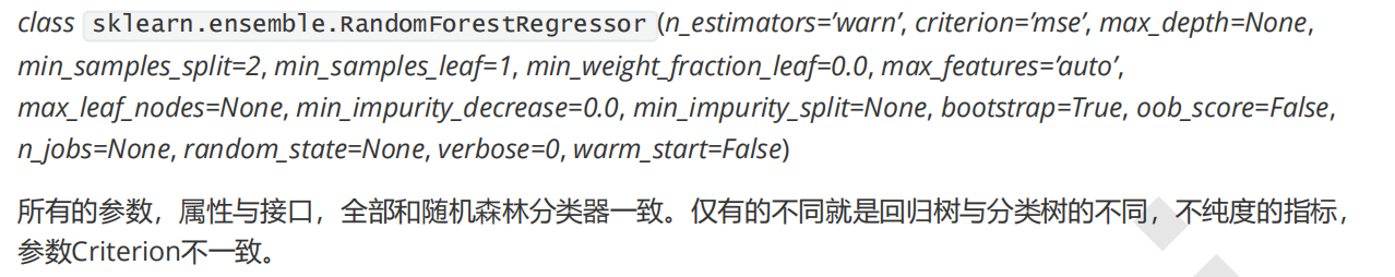
criterion:
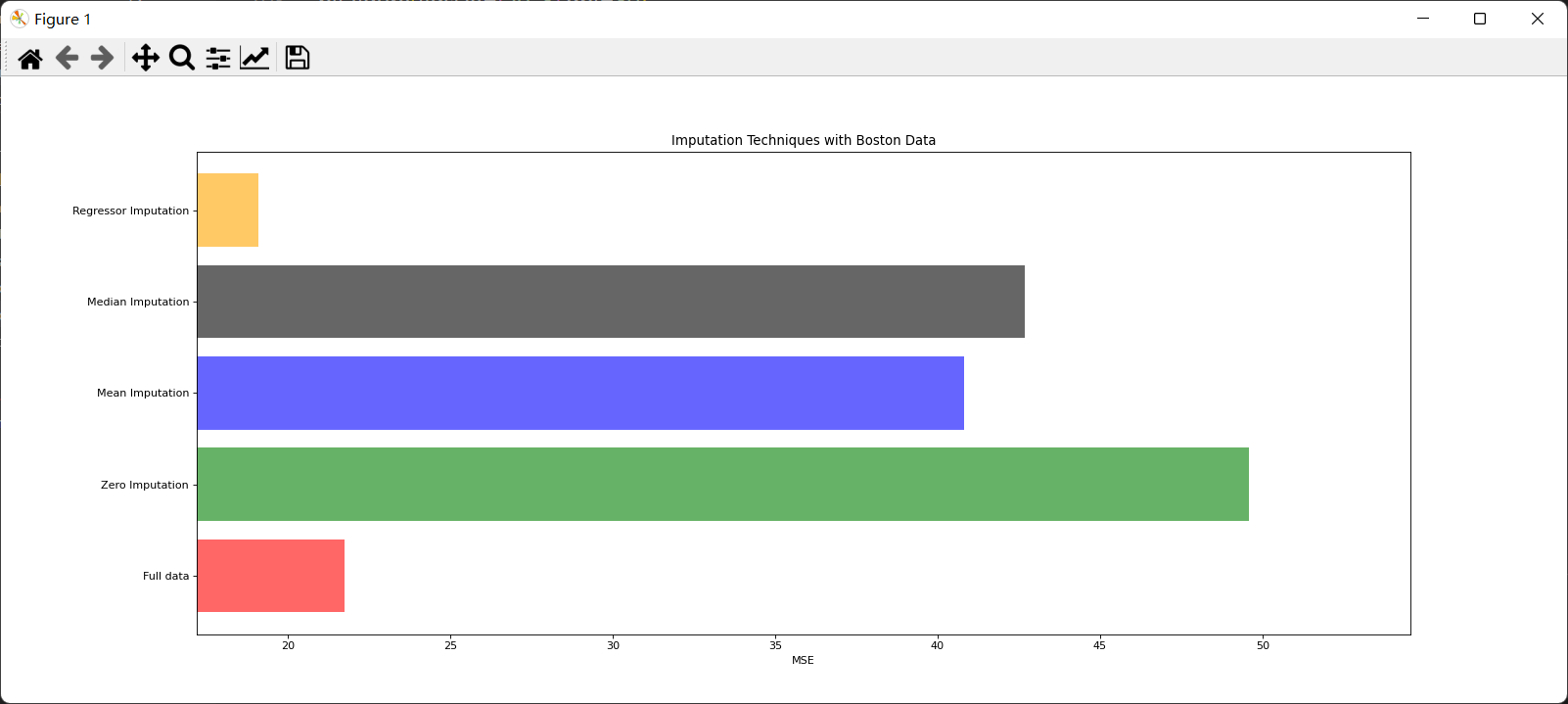
3.2 filling missing values with random forest regression
For a data with n features, where feature t has missing values, we take feature t as a label, and the other n-1 features and the original label form a new feature matrix. For T, there is no missing part, that is, our Y_test, this part of the data has both labels and features, and the missing part has only features and no labels, which is the part we need to predict.
Other n-1 features corresponding to the value of feature T not missing + original label: X_train
Value of characteristic T not missing: Y_train
Other n-1 features corresponding to the missing value of feature T + original label: X_test
Missing value of characteristic T: unknown, we need to predict Y_test
import numpy as np
import pandas as pd
import matplotlib.pyplot as plt
from pandas.core.frame import DataFrame
from sklearn.datasets import load_boston
from sklearn.impute import SimpleImputer
from sklearn.ensemble import RandomForestRegressor
from sklearn.model_selection import cross_val_score

boston=load_boston()
# print(boston)
# print(boston.data.shape)

#After storing the complete data set, the missing data set will be processed and filled, and then compared with the original data set
x_full,y_full=boston.data,boston.target #Storing original data and characteristics
n_samples=x_full.shape[0]#Record the number of complete samples
n_features=x_full.shape[1]#Record the number of complete features

#Put missing values for full data
#Determine the proportion of missing values, here we assume 50%
rng=np.random.RandomState(0)#Determine a random pattern
missing_rate=0.5
n_missing_samples=int(np.floor(n_samples*n_features*missing_rate))#Round down, resulting in the total number of missing data
# print(n_missing_samples)

#The generated missing values are distributed in each row and column of the data
miss_features=rng.randint(0,n_features,n_missing_samples) #The three parameters are the number of lower and upper limits in turn
miss_samples=rng.randint(0,n_samples,n_missing_samples)

#If the random number taken out is less than the sample size, the choice method can be used
#missing_samples = rng.choice(n_samples,n_missing_samples,replace=False) #The number of random fetches required when the parameters from left to right are the maximum will not be repeated to ensure more scattered data

#Create missing data
#Operate after copying the original complete data
x_missing=x_full.copy()
y_missing=y_full.copy()
#Replace a part of the complete data with a missing value
x_missing[miss_samples,miss_features]=np.nan
#Convert to dataframe to facilitate subsequent operations
x_missing=DataFrame(x_missing)
# print(x_missing)

#Filling missing values with mean
imp_mean=SimpleImputer(missing_values=np.nan,strategy='mean')#instantiation
x_missing_mean = imp_mean.fit_transform(x_missing) #fit_transform training + export predict
#Check whether the filling is completed
# print(pd.DataFrame(x_missing_mean).isnull().sum())

#Fill missing values with median
imp_median=SimpleImputer(missing_values=np.nan,strategy='median')#instantiation
x_missing_median = imp_median.fit_transform(x_missing) #fit_transform training + export predict
#Check whether the filling is completed
# print(pd.DataFrame(x_missing_median).isnull().sum())

#Fill with 0
imp_0 = SimpleImputer(missing_values=np.nan, strategy="constant",fill_value=0)
x_missing_0 = imp_0.fit_transform(x_missing)
#Check whether the filling is completed
# print(pd.DataFrame(x_missing_0).isnull().sum())

#Filling missing values with random forests
x_missing_reg=x_missing.copy()#Replicate matrices that require regression to fill in missing values
#The essence of finding out the order of the corresponding eigenvalues from small to large is to find the index and fill it from the one with the most missing values
sortindex=np.argsort(x_missing_reg.isnull().sum(axis=0)).values #argsort returns the index and uses values to fetch the data
#Traversal fill missing values
for i in sortindex:
    #Build a new feature matrix (features not selected to be filled + original labels) and a new label (features selected to be filled)
    df=x_missing_reg
    fillc=df.iloc[:,i]
    #New characteristic matrix
    df=pd.concat([df.iloc[:,df.columns!=i],pd.DataFrame(y_full)],axis=1) #Left right connection
    #In the new characteristic matrix, the columns with missing values are filled with 0
    df_0 =SimpleImputer(missing_values=np.nan,strategy='constant',fill_value=0).fit_transform(df)
    #Find training set and test set
    Ytrain = fillc[fillc.notnull()] #Non empty in features selected to fill
    Ytest = fillc[fillc.isnull()]     #For those values that do not exist in the selected features to be filled, we need not the value of ytest, but its index
    Xtrain = df_0[Ytrain.index,:] #On the new characteristic matrix, the record corresponding to the selected non null value
    Xtest = df_0[Ytest.index,:]    #On the new feature matrix, the record corresponding to the selected feature null value

    #Filling missing values using random forests
    rfc = RandomForestRegressor(n_estimators=100)
    rfc = rfc.fit(Xtrain, Ytrain)
    Ypredict = rfc.predict(Xtest)#Get the prediction results

    #Fill the filled features into the original feature matrix
    x_missing_reg.loc[x_missing_reg.iloc[:,i].isnull(),i]=Ypredict  #First, use iloc to find the row index of nan

# print(x_missing_reg.isnull().sum())

#All data were modeled and MSE results were obtained
X = [x_full,x_missing_0,x_missing_mean,x_missing_median,x_missing_reg]
mse = []
std = []
for x in X:
    estimator = RandomForestRegressor()
    scores = cross_val_score(estimator,x,y_full,scoring='neg_mean_squared_error', cv=5).mean()#Score with negative mean square error
    mse.append(scores * -1)#Turn the result to positive
print(*zip(['x_full','x_missing_0','x_missing_mean','x_missing_median','x_missing_reg'],mse))#The smaller the better

#mapping
x_labels = ['Full data','Zero Imputation','Mean Imputation','Median Imputation','Regressor Imputation']
colors = ['r', 'g', 'b','black', 'orange']
plt.figure(figsize=(20, 8),dpi=80)
ax = plt.subplot(111) #Add subgraphs to prepare for subsequent functionalization
for i in np.arange(len(mse)):
    ax.barh(i, mse[i],color=colors[i], alpha=0.6, align='center') #Draw the bar chart horizontally in the center
ax.set_title('Imputation Techniques with Boston Data')
ax.set_xlim(left=np.min(mse) * 0.9,right=np.max(mse) * 1.1)#The x-axis of the limited range is mse value
ax.set_yticks(np.arange(len(mse)))#Set y scale
ax.set_xlabel('MSE')
ax.set_yticklabels(x_labels)#Change y's scale
plt.show()
4 basic idea of machine learning parameter adjustment
4.1 related concepts
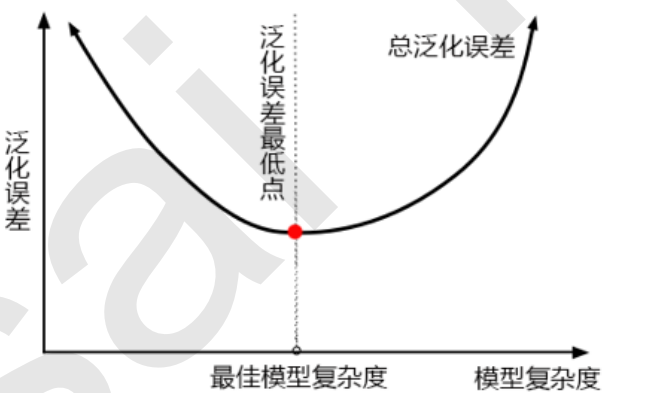
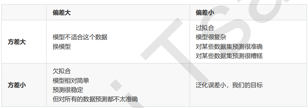
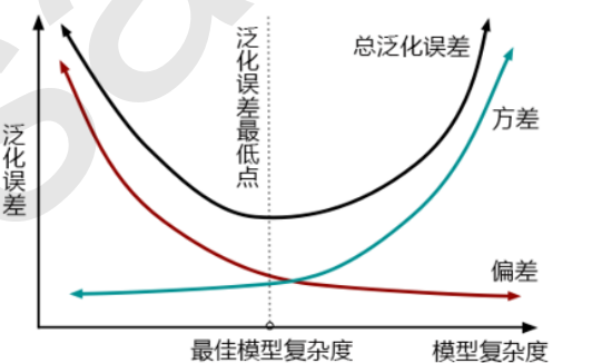
The first step in model tuning is to find the right goal: what are we going to do? Generally speaking, this goal is to improve the evaluation index of a model. For example, for random forests, what we want to improve is the accuracy of the model on unknown data (measured by score or oob_score_). To find this goal, we need to think: what factors affect the accuracy of the model on unknown data? In machine learning, the index we use to measure the accuracy of the model on unknown data is called generalization error.
4.2 examples
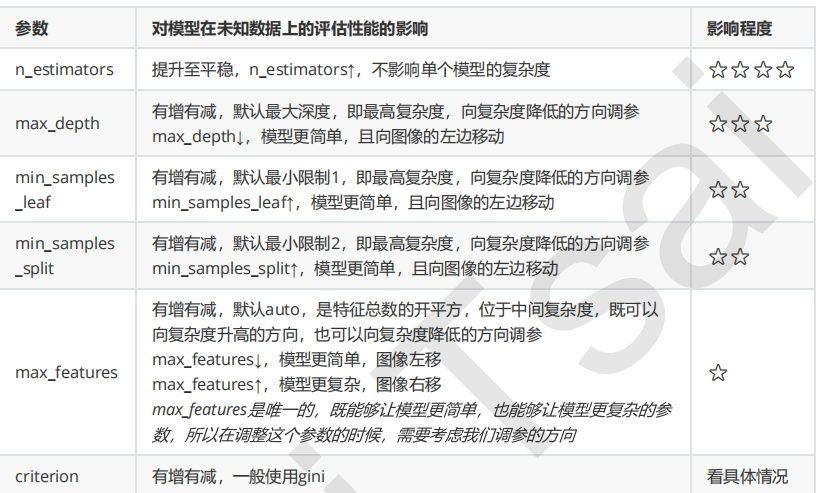
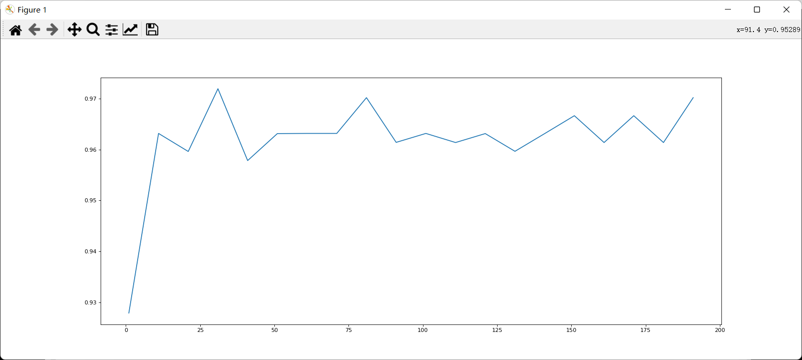
View n_ The learning curve of estimators.

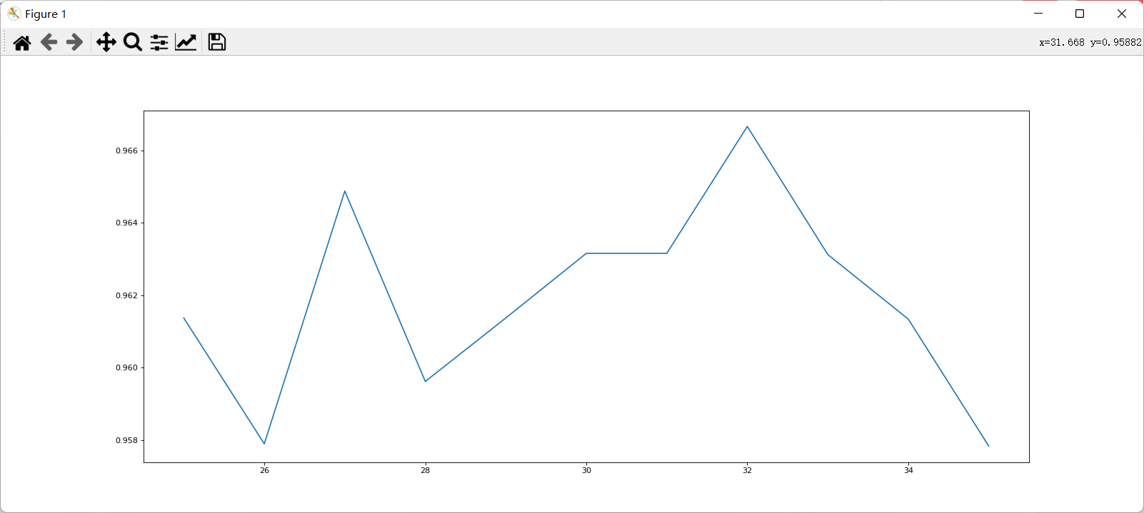
After determining the good range, further refine the learning curve.
Because the division of each training set and test set is different, the performance after refinement may be worse than before, but in general, the refined curve can provide a more accurate parameter selection range. After determining the number of base evaluators, further use grid search to find other appropriate parameters.

Max is modulated_ After depth, the accuracy of the model increases, so the model is on the right side of the generalization complexity.


Min at this time_ samples_ Split reduces the accuracy, so the parameter is not set.
Adjust random_state

The accuracy is improved.

The complete code is as follows
from sklearn.datasets import load_breast_cancer
from sklearn.ensemble import RandomForestClassifier
from sklearn.model_selection import GridSearchCV
from sklearn.model_selection import cross_val_score
import matplotlib.pyplot as plt
import pandas as pd
import numpy as np
data = load_breast_cancer()
#preliminary estimates
# scorel = []
# for i in range(0,200,10):
# rfc=RandomForestClassifier(n_estimators=i+1)
# score=cross_val_score(rfc,data.data,data.target,cv=10).mean()
# scorel.append(score)
# print(max(scorel),(scorel.index(max(scorel))*10)+1)
# plt.figure(figsize=[20,8],dpi=80)
# plt.plot(range(1,201,10),scorel)
# plt.show()
#Refined estimation
# scorel = []
# for i in range(25,36):
# rfc=RandomForestClassifier(n_estimators=i+1)
# score=cross_val_score(rfc,data.data,data.target,cv=10).mean()
# scorel.append(score)
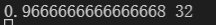
# print(max(scorel),([*range(25,36)][scorel.index(max(scorel))])) #Take the index corresponding to the maximum value in the range of 30-39
# plt.figure(figsize=[20,8],dpi=80)
# plt.plot(range(25,36),scorel)
# plt.show()
#Adjust max_depth
# param_grid = {'max_depth':np.arange(1, 20, 1)}
# Generally based on the size of the data to carry out a test, breast cancer data is very small, so you can use 1~10, or 1~20 test.
# However, for large data like digital recognition, we should try 30 ~ 50 layers of depth (maybe not enough)
# We should draw a learning curve to observe the influence of depth on the model
# rfc = RandomForestClassifier(n_estimators=32)
# GS = GridSearchCV(rfc,param_grid,cv=10)
# GS.fit(data.data,data.target)
# print(GS.best_params_,GS.best_score_)
#Adjust max_features
#Now that the model is on the right side of the image, we need lower complexity
#max_ The default minimum value of features is sqrt(n_features), so we use twice this value as the maximum value of the tuning range.
# param_grid = {'max_features':np.arange(1,10,1)}
# rfc = RandomForestClassifier(n_estimators=32,max_depth=11)
# GS = GridSearchCV(rfc,param_grid,cv=10)
# GS.fit(data.data,data.target)
# print(GS.best_params_,GS.best_score_)
#Adjustment min_samples_leaf
#For min_samples_split and min_samples_leaf is generally increased by 10 or 20 from their minimum value
#In the face of high-dimensional and high sample size data, if you are not confident, you can also directly + 50. For large data, you may need a range of 200 ~ 300
#If you find that the accuracy can not be improved in any case during adjustment, you can rest assured and boldly adjust a large data to greatly limit the complexity of the model
# param_grid={'min_samples_leaf':np.arange(1, 1+10, 1)}
# rfc = RandomForestClassifier(n_estimators=32,max_depth=11,max_features=7)
# GS = GridSearchCV(rfc,param_grid,cv=10)
# GS.fit(data.data,data.target)
# print(GS.best_params_,GS.best_score_)
#Adjust random_state
# param_grid={'random_state':np.arange(20,150)}
# rfc = RandomForestClassifier(n_estimators=32,max_depth=11,max_features=7)
# GS = GridSearchCV(rfc,param_grid,cv=10)
# GS.fit(data.data,data.target)
# print(GS.best_params_,GS.best_score_)
#Determine final parameters
rfc = RandomForestClassifier(n_estimators=39,max_depth=11,max_features=7,random_state=66)
score = cross_val_score(rfc,data.data,data.target,cv=10)
print(score)