Data links and codes: https://pan.baidu.com/s/19Rj_kP2iJ0szS6l2IWg6FQ
Extraction code: ezbd
1. Data analysis
Dataset divorce Xlsx, let's take a look at the data description first. In short, each dimension corresponds to a questionnaire question. As shown in the figure
Libraries to be imported:
import pandas as pd
import numpy as np
import matplotlib.pyplot as plt
import seaborn as sns  # It is convenient to use this library to draw the data distribution feature map. pip install seaborn is OK
%matplotlib inline
plt.rcParams['font.sans-serif'] = ['KaiTi']  # Specifies the default font
from sklearn.model_selection import cross_val_score  # k-fold cross validation
from sklearn.model_selection import train_test_split   # Import modules that automatically generate training sets and test sets
from sklearn.metrics import classification_report   # Import prediction result evaluation module
from sklearn.linear_model import LogisticRegression  # logistic regression
from sklearn.metrics import confusion_matrix  # Confusion matrix
from sklearn.ensemble import RandomForestClassifier  # Random forest classification
from sklearn.tree import DecisionTreeClassifier  # Decision tree
from sklearn.neighbors import KNeighborsClassifier  # KNN
from sklearn import svm   # Support vector machine
Read in data
data_train = pd.read_excel('divorce.xlsx')
# Let pandas tell us some information first. It is found that there are no missing values, so there is no need to fill in the missing values
data_train.info()
print(data_train)
data_train.describe()
<class 'pandas.core.frame.DataFrame'>
RangeIndex: 170 entries, 0 to 169
Data columns (total 55 columns):
Atr1 170 non-null int64
Atr2 170 non-null int64
Atr3 170 non-null int64
Atr4 170 non-null int64
Atr5 170 non-null int64
Atr6 170 non-null int64
Atr7 170 non-null int64
Atr8 170 non-null int64
Atr9 170 non-null int64
Atr10 170 non-null int64
Atr11 170 non-null int64
Atr12 170 non-null int64
Atr13 170 non-null int64
Atr14 170 non-null int64
Atr15 170 non-null int64
Atr16 170 non-null int64
Atr17 170 non-null int64
Atr18 170 non-null int64
Atr19 170 non-null int64
Atr20 170 non-null int64
Atr21 170 non-null int64
Atr22 170 non-null int64
Atr23 170 non-null int64
Atr24 170 non-null int64
Atr25 170 non-null int64
Atr26 170 non-null int64
Atr27 170 non-null int64
Atr28 170 non-null int64
Atr29 170 non-null int64
Atr30 170 non-null int64
Atr31 170 non-null int64
Atr32 170 non-null int64
Atr33 170 non-null int64
Atr34 170 non-null int64
Atr35 170 non-null int64
Atr36 170 non-null int64
Atr37 170 non-null int64
Atr38 170 non-null int64
Atr39 170 non-null int64
Atr40 170 non-null int64
Atr41 170 non-null int64
Atr42 170 non-null int64
Atr43 170 non-null int64
Atr44 170 non-null int64
Atr45 170 non-null int64
Atr46 170 non-null int64
Atr47 170 non-null int64
Atr48 170 non-null int64
Atr49 170 non-null int64
Atr50 170 non-null int64
Atr51 170 non-null int64
Atr52 170 non-null int64
Atr53 170 non-null int64
Atr54 170 non-null int64
Class 170 non-null int64
dtypes: int64(55)
memory usage: 73.2 KB
Atr1 Atr2 Atr3 Atr4 Atr5 Atr6 Atr7 Atr8 Atr9 Atr10 ... Atr46 \
0 2 2 4 1 0 0 0 0 0 0 ... 2
1 4 4 4 4 4 0 0 4 4 4 ... 2
2 2 2 2 2 1 3 2 1 1 2 ... 3
3 3 2 3 2 3 3 3 3 3 3 ... 2
4 2 2 1 1 1 1 0 0 0 0 ... 2
.. ... ... ... ... ... ... ... ... ... ... ... ...
165 0 0 0 0 0 0 0 0 0 0 ... 1
166 0 0 0 0 0 0 0 0 0 0 ... 4
167 1 1 0 0 0 0 0 0 0 1 ... 3
168 0 0 0 0 0 0 0 0 0 0 ... 3
169 0 0 0 0 0 0 0 1 0 0 ... 3
Atr47 Atr48 Atr49 Atr50 Atr51 Atr52 Atr53 Atr54 Class
0 1 3 3 3 2 3 2 1 1
1 2 3 4 4 4 4 2 2 1
2 2 3 1 1 1 2 2 2 1
3 2 3 3 3 3 2 2 2 1
4 1 2 3 2 2 2 1 0 1
.. ... ... ... ... ... ... ... ... ...
165 0 4 1 1 4 2 2 2 0
166 1 2 2 2 2 3 2 2 0
167 0 2 0 1 1 3 0 0 0
168 3 2 2 3 2 4 3 1 0
169 4 4 0 1 3 3 3 1 0
[170 rows x 55 columns]
Out[23]:
| Atr1 | Atr2 | Atr3 | Atr4 | Atr5 | Atr6 | Atr7 | Atr8 | Atr9 | Atr10 | ... | Atr46 | Atr47 | Atr48 | Atr49 | Atr50 | Atr51 | Atr52 | Atr53 | Atr54 | Class | |
|---|---|---|---|---|---|---|---|---|---|---|---|---|---|---|---|---|---|---|---|---|---|
| count | 170.000000 | 170.000000 | 170.000000 | 170.000000 | 170.000000 | 170.000000 | 170.000000 | 170.000000 | 170.000000 | 170.000000 | ... | 170.000000 | 170.000000 | 170.000000 | 170.000000 | 170.000000 | 170.000000 | 170.000000 | 170.000000 | 170.000000 | 170.000000 |
| mean | 1.776471 | 1.652941 | 1.764706 | 1.482353 | 1.541176 | 0.747059 | 0.494118 | 1.452941 | 1.458824 | 1.576471 | ... | 2.552941 | 2.270588 | 2.741176 | 2.382353 | 2.429412 | 2.476471 | 2.517647 | 2.241176 | 2.011765 | 0.494118 |
| std | 1.627257 | 1.468654 | 1.415444 | 1.504327 | 1.632169 | 0.904046 | 0.898698 | 1.546371 | 1.557976 | 1.421529 | ... | 1.371786 | 1.586841 | 1.137348 | 1.511587 | 1.405090 | 1.260238 | 1.476537 | 1.505634 | 1.667611 | 0.501442 |
| min | 0.000000 | 0.000000 | 0.000000 | 0.000000 | 0.000000 | 0.000000 | 0.000000 | 0.000000 | 0.000000 | 0.000000 | ... | 0.000000 | 0.000000 | 0.000000 | 0.000000 | 0.000000 | 0.000000 | 0.000000 | 0.000000 | 0.000000 | 0.000000 |
| 25% | 0.000000 | 0.000000 | 0.000000 | 0.000000 | 0.000000 | 0.000000 | 0.000000 | 0.000000 | 0.000000 | 0.000000 | ... | 2.000000 | 1.000000 | 2.000000 | 1.000000 | 1.000000 | 2.000000 | 1.000000 | 1.000000 | 0.000000 | 0.000000 |
| 50% | 2.000000 | 2.000000 | 2.000000 | 1.000000 | 1.000000 | 0.000000 | 0.000000 | 1.000000 | 1.000000 | 2.000000 | ... | 3.000000 | 2.000000 | 3.000000 | 3.000000 | 2.000000 | 3.000000 | 3.000000 | 2.000000 | 2.000000 | 0.000000 |
| 75% | 3.000000 | 3.000000 | 3.000000 | 3.000000 | 3.000000 | 1.000000 | 1.000000 | 3.000000 | 3.000000 | 3.000000 | ... | 4.000000 | 4.000000 | 4.000000 | 4.000000 | 4.000000 | 4.000000 | 4.000000 | 4.000000 | 4.000000 | 1.000000 |
| max | 4.000000 | 4.000000 | 4.000000 | 4.000000 | 4.000000 | 4.000000 | 4.000000 | 4.000000 | 4.000000 | 4.000000 | ... | 4.000000 | 4.000000 | 4.000000 | 4.000000 | 4.000000 | 4.000000 | 4.000000 | 4.000000 | 4.000000 | 1.000000 |
8 rows × 55 columns
No missing values were found,
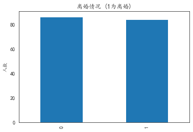
Look at the number of divorced and non divorced people in the data.
# Look at the number of divorced and non divorced people in the data
data_train['Class'].value_counts().plot(kind='bar')
plt.title(u"Divorce (1 For divorce)") # puts a title on our graph
plt.ylabel(u"Number of people")

'''We found that the number of positive and negative samples was basically the same
Text(0, 0.5, 'Number of people')
View data dependencies
# Since there are 50 multi-dimensional features in total, the importance of some features is not so great corresponding to the different answers to 50 questions
# Correlation of each eigenvector
print(data_train.corr())
# Make correlation matrix
plt.figure(figsize=(48, 36))
sns.set_style("whitegrid")
sns.heatmap(data_train.corr(),annot=True, cmap='Blues', vmin = 0.0, vmax = 1 ,linewidths=1)

'''It is found that many data have strong correlation'''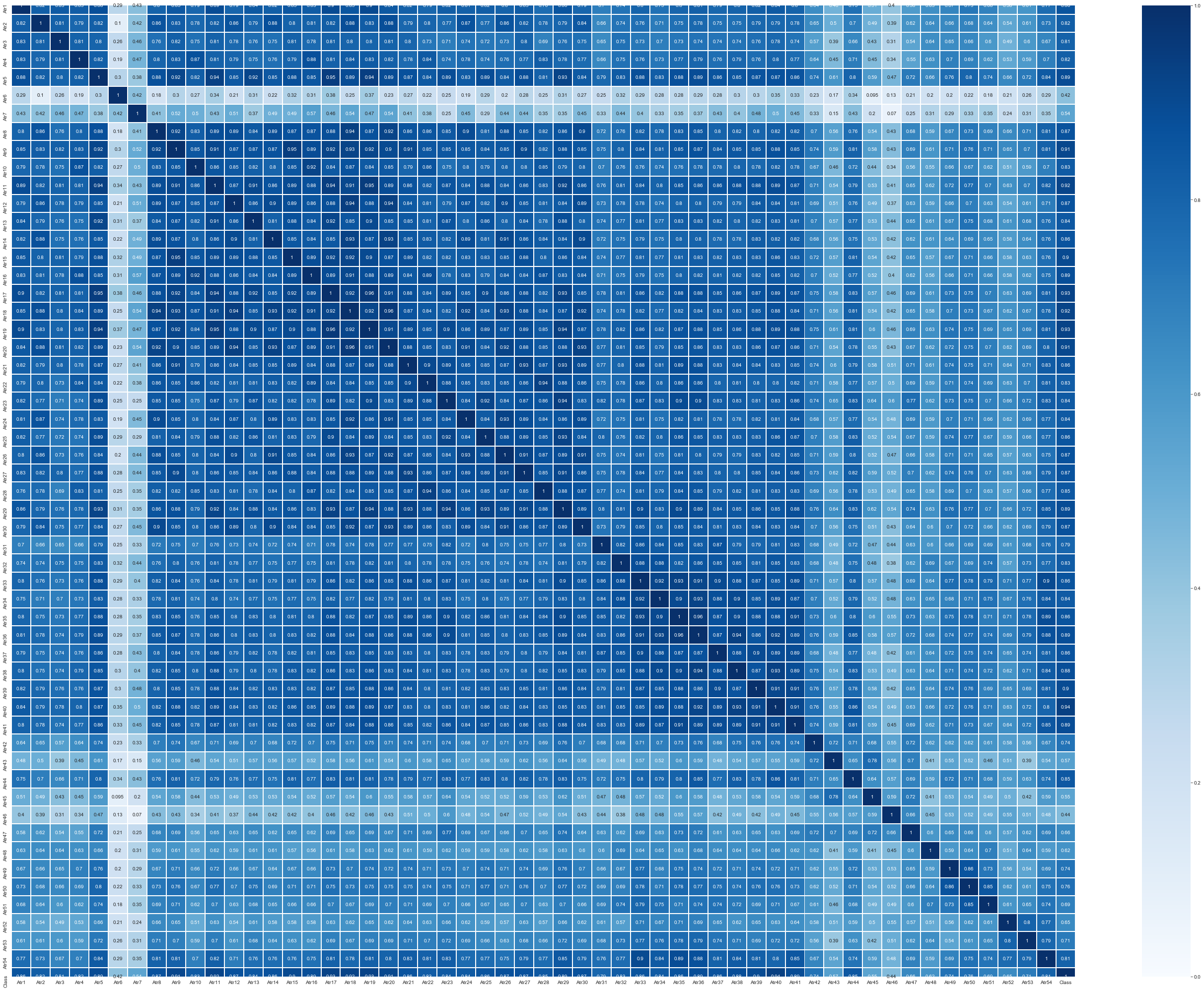
Look at the variance again
# covariance matrix
print(data_train.cov())
xfc = data_train.cov()
cov = []
for i in range(data_train.shape[1]-1):
    cov.append(xfc.iloc[i, i])
plt.bar(data_train.columns[:-1], np.array(cov))
plt.title(u"Characteristic variance")
plt.xlabel("features")
plt.ylabel(u"variance")
plt.show()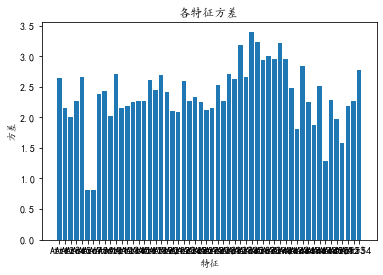
In general, the data is perfect and there are no missing values, so there is no need to fill in the missing values. Since each data is a number of 0 ~ 4, which represents different answers to the question, it is not necessary to normalize and standardize the data, nor do we need to carry out one-hot operation. The correlation between some features is relatively high, so a dimension reduction operation can be considered. However, based on the special property that each attribute corresponds to a survey problem, each row of data obtained by dimension reduction methods such as PCA and SVD can be regarded as the projection coordinates of the original m pieces of data on the new k dimensions, This changes the special property that each feature corresponds to a survey problem, and we hope to select some important problems from these problems to simplify the model. Therefore, it is not suitable to use dimensionality reduction methods such as PCA and SVD for dimensionality reduction. Therefore, it is necessary to simplify the model by feature selection.
Try the model first. Try it here.
# Logistic regression, using 10 fold cross validation, evaluated with accuracy, found that the curve converged when C=0.4.
C_params = np.linspace(0.01, 1, 100)
test_scores = []
for c in C_params:
    clf = LogisticRegression(C=c, penalty='l2', tol=1e-6)
    test_score = cross_val_score(clf, train_X, train_y, cv=10, scoring='accuracy')
    test_scores.append(np.mean(test_score))

plt.plot(C_params, test_scores)
plt.title("adjustment LR Penalty coefficient c")
plt.xlabel('Penalty coefficient C')
plt.ylabel('10 Accuracy of cross validation')
plt.show()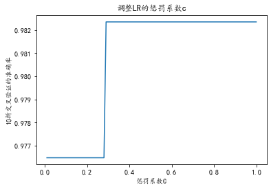
The optimal parameter C=0.4 and the accuracy is 0.982
# Predict, evaluate and draw confusion matrix
# The data set was divided into 37 points, 7 training and 3 prediction
clf = LogisticRegression(C=0.4, penalty='l2', tol=1e-6)
X_train, X_test, y_train, y_test = train_test_split(train_X, train_y, test_size=0.3)
clf.fit(X_train, y_train)
print("The prediction and evaluation results are as follows:\n", classification_report(y_test, clf.predict(X_test)))
The prediction and evaluation results are as follows:
precision recall f1-score support
0 0.97 1.00 0.98 28
1 1.00 0.96 0.98 23
accuracy 0.98 51
macro avg 0.98 0.98 0.98 51
weighted avg 0.98 0.98 0.98 51from sklearn import svm # Support vector machine
from sklearn.model_selection import GridSearchCV # Grid search tuning
# Grid search parameter adjustment of SVM
param = {'kernel': ['rbf', 'poly'], 'C': np.linspace(1, 100, 100)}
grid = GridSearchCV(svm.SVC(), param_grid=param, cv=10)
grid.fit(train_X, train_y)
print('best params:', grid.best_params_,'best score:', grid.best_score_) # The optimal parameters and scores are obtained
means = grid.cv_results_['mean_test_score']
params = grid.cv_results_['params']
hhhh = pd.concat([pd.DataFrame(params), pd.DataFrame({'score': means})], axis=1)
hhhh
# for mean, param in zip(means, params):
# print("parameter: {} \ t test_score: {} \ t".format(param, mean))best params: {'C': 2.0, 'kernel': 'rbf'} best score: 0.9823529411764707feature selection
Please refer to: https://www.cnblogs.com/stevenlk/p/6543628.html
Here we learn from the content in this link.
It has been analyzed in the data analysis stage that each attribute of divorce prediction problem corresponds to a survey problem. Dimensionality reduction methods such as PCA and SVD will change this special property. In order to select some important problems from these problems to simplify and optimize the model, feature selection is needed.
Feature selection has two main purposes: one is to reduce the number of features and dimension, so as to enhance the generalization ability of the model and reduce over fitting; The second is to enhance the understanding between features and eigenvalues. According to the form of feature selection, feature selection methods can be divided into the following three types:
- Filter: filter method, which scores each feature according to divergence or correlation, sets the threshold or the number of thresholds to be selected, and selects features.
- Wrapper: packaging method, which selects or excludes several features each time according to the objective function (usually the prediction effect score). A basic model is used for multiple rounds of training. After each round of training, the features of several weight coefficients are removed, and then the next round of training is carried out based on the new feature set.
- Embedded: embedding method. Firstly, some machine learning algorithms and models are used for training to obtain the weight coefficients of each feature, and the features are selected from large to small according to the coefficients. It is similar to the Filter method, but it determines the advantages and disadvantages of features through training.
It can be seen from Figure 3 in the data analysis stage that the variance of each dimension is large, so the data is divergent, so the Filter method is not suitable for filtering low variance data. If the Wrapper is used for feature selection through recursion, this example is a set of features with a number of 54, with a total of 254-1 non empty subsets. Therefore, the time complexity and amount of calculation are huge, and it is not suitable for this example.
Since the model of the logistic regression contains the first mock exam W1~Wn of each feature, it is consistent with the characteristics of Embedded method. Based on the adjusted parameters of the logistic regression model, the embedded method is used for feature selection
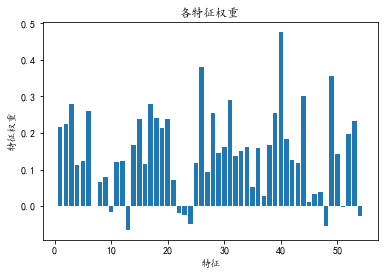
# Find the six features with the largest weight, and their subscripts are 2 30 43 48 25 39 respectively
clf = LogisticRegression(C=0.4, penalty='l2', tol=1e-6)
clf.fit(train_X, train_y)
weight_arr = np.array(clf.coef_).reshape(-1)
print('10 characteristic subscripts with the largest weight:', weight_arr.argsort()[-10:])
print('Weight of each feature', clf.coef_)
plt.bar(range(1, train_X.shape[1]+1), weight_arr)
plt.title(u"Weight of each feature")
plt.xlabel("features")
plt.ylabel(u"Feature weight")
plt.show()
Six feature subscripts with the largest weight: [38 27 5 16 2 30 43 48 25 39] Weight of each feature [[ 2.17720972e-01 2.24766611e-01 2.80719097e-01 1.13008502e-01 1.22699281e-01 2.60222839e-01 -2.21849802e-04 6.48332841e-02 7.97345462e-02 -1.58821783e-02 1.20942969e-01 1.24425583e-01 -6.46131183e-02 1.67072655e-01 2.37785099e-01 1.14999839e-01 2.78684197e-01 2.41468503e-01 2.14227280e-01 2.39629025e-01 7.05548979e-02 -2.00206891e-02 -2.57268937e-02 -4.95804574e-02 1.18052477e-01 3.81350374e-01 9.34487757e-02 2.55759482e-01 1.44724330e-01 1.62397921e-01 2.90033904e-01 1.38180436e-01 1.50782978e-01 1.61433520e-01 5.26107564e-02 1.58250954e-01 2.66690085e-02 1.65857456e-01 2.54333885e-01 4.76657143e-01 1.84107213e-01 1.26628270e-01 1.17035298e-01 3.02576017e-01 1.21383739e-02 3.40128328e-02 3.84344718e-02 -5.41742213e-02 3.56737710e-01 1.42873105e-01 -3.61608478e-03 1.97740815e-01 2.31508643e-01 -2.79129682e-02]]
# Next, we iterate and optimize. The n features with the largest weight are the ordinates, and the accuracy of 10 fold cross validation is the abscissa. When we find several specific parameters, the accuracy is the highest
# It is found that when the number of features is 10, the accuracy is the highest, 0.994. The subscripts of these 10 features are 38 27 5 16 2 30 43 48 25 39 respectively
clf = LogisticRegression(C=0.4, penalty='l2', tol=1e-6)
clf.fit(train_X, train_y)
weight_arr = np.array(clf.coef_).reshape(-1)
weight_arr_arg = weight_arr.argsort()
test_scores = []
for i in range(3, 20):
    clf = LogisticRegression(C=0.4, penalty='l2', tol=1e-6)
    test_score = cross_val_score(clf, train_X[:, weight_arr_arg[-i:]], train_y, cv=10, scoring='accuracy')
    test_scores.append(np.mean(test_score))

plt.plot(range(3, 20), test_scores)
plt.title("Number of features - accuracy chart")
plt.xlabel("Select the front with the largest weight n Number of features")
plt.ylabel("10 Accuracy of cross validation")
plt.show()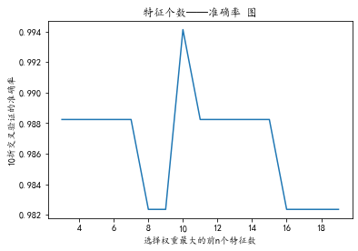
When only the first 4 ~ 6 features with the largest weight are selected, the accuracy of cross validation is improved from 0.982 to 0.988. When the first 10 features with the largest weight are selected, the accuracy of cross validation is improved to the highest - 0.994.
The problems corresponding to these 10 features are as follows:
| question | feature | Weight |
| We're just starting a discussion before I know what's going on | 40 | 0.47665714 |
| I know my spouse's basic anxieties. | 26 | 0.38135037 |
| I have nothing to do with what I've been accused of. | 49 | 0.35673771 |
| Sometimes I think it's good for me to leave home for a while. | 44 | 0.30257602 |
| I feel aggressive when I argue with my spouse. | 31 | 0.2900339 |
| When we need it, we can take our discussions with my spouse from the beginning and correct it. | 3 | 0.2807191 |
| We share the same views about being happy in our life with my spouse | 17 | 0.2786842 |
| We don't have time at home as partners. | 6 | 0.26022284 |
| I know my spouse's hopes and wishes. | 28 | 0.25575948 |
| Our discussions often occur suddenly. | 39 | 0.25433389 |
6. The accuracy and F1 score of the feature model reach 0.98, which is almost the same as that of the previous model trained with all features, greatly reducing the data dimension of the training model, that is, reducing the number of questions to be filled in by the respondents in the practical application of the model from the original 54 questions to 6 or 10 questions, This is convenient for the practical application of the model.
Finally, the trained model is obtained and saved as LR Pkl file
from sklearn.externals import joblib  # Save model

train_X = train_X[:, [2, 30, 43, 48, 25, 39]]
clf = LogisticRegression(C=0.4, penalty='l2', tol=1e-6)
test_score = cross_val_score(clf, train_X, train_y, cv=10, scoring='accuracy')
print('accuracy: ', np.mean(test_score))
clf.fit(train_X, train_y)
# Save model
joblib.dump(clf, 'divorce LR.pkl')
Finally, I made a GUI interface (although it doesn't look very good, I'm too lazy to polish), which is convenient to use.
Brothers can keep it and use it when necessary. Hahaha.
import pyefun.wxefun as wx  # GUI design library. This library is quite convenient to use. pip install pyefun
from sklearn.externals import joblib  # Save model

class Window 1(wx.window):
    def __init__(self):
        self.Initialization interface()
        self.clf = joblib.load('divorce LR.pkl')
        self.dic = {'never': 0, 'very seldom': 1, 'Sometimes': 2, 'often': 3, 'always': 4}
        self.result_dic = {0: 'No divorce', 1: 'divorce'}
        print("Loading model completed")

    def Initialization interface(self):
        #########The following is the created component code#########
        wx.window.__init__(self, None, title='Divorce test system by Ahau ', size=(742, 532), name='frame', style=541072896)
        self.container = wx.container(self)
        self.Centre()
        self.Window 1 = self

        self.Label 1 = wx.label(self.container, size=(582, 47), pos=(23, 22), label='This system is only for married people!', name='staticText', style=2321)
        self.Label 1.typeface = wx.Font(22, 74, 90, 400, False, 'Microsoft YaHei UI', 28)
        self.Label 2 = wx.label(self.container, size=(479, 37), pos=(17, 91), label="When necessary,I can discuss the problem with my spouse from the beginning and correct it.", name='staticText', style=2321)
        self.Label 2.typeface = wx.Font(12, 74, 90, 400, False, 'Microsoft YaHei UI', -1)
        self.Combo box 1 = wx.combo box(self.container, value='', pos=(535, 91), name='comboBox', choices=[], style=16)
        self.Combo box 1.SetSize((60, 37))
        self.Combo box 1.typeface = wx.Font(12, 74, 90, 400, False, 'Microsoft YaHei UI', -1)
        self.Combo box 1.background color  = (255, 255, 255, 255)
        self.Combo box 1.Join project(['never', 'very seldom', 'Sometimes', 'often', 'always'])
        self.Label 3 = wx.label(self.container, size=(479, 37), pos=(17, 141), label="When I argue with my spouse, I feel very aggressive.", name='staticText', style=2321)
        self.Label 3.typeface = wx.Font(12, 74, 90, 400, False, 'Microsoft YaHei UI', -1)
        self.Combo box 3 = wx.combo box(self.container, value='', pos=(535, 141), name='comboBox', choices=[], style=16)
        self.Combo box 3.SetSize((60, 37))
        self.Combo box 3.typeface = wx.Font(12, 74, 90, 400, False, 'Microsoft YaHei UI', -1)
        self.Combo box 3.background color  = (255, 255, 255, 255)
        self.Combo box 3.Add project(['never', 'very seldom', 'Sometimes', 'often', 'always'])
        self.Label 4 = wx.label(self.container, size=(479, 37), pos=(17, 191), label='Sometimes I think it's good for me to leave home for a while.', name='staticText', style=2321)
        self.Label 4.typeface = wx.Font(12, 74, 90, 400, False, 'Microsoft YaHei UI', -1)
        self.Combo box 4 = wx.Combo box(self.container, value='', pos=(535, 191), name='comboBox', choices=[], style=16)
        self.Combo box 4.SetSize((60, 37))
        self.Combo box 4.typeface = wx.Font(12, 74, 90, 400, False, 'Microsoft YaHei UI', -1)
        self.Combo box 4.background color  = (255, 255, 255, 255)
        self.Combo box 4.Add project(['never', 'very seldom', 'Sometimes', 'often', 'always'])
        self.Label 5 = wx.label(self.container, size=(479, 37), pos=(17, 241), label="Where I have been accused by my spouse, I don't want to correct it", name='staticText', style=2321)
        self.Label 5.typeface = wx.Font(12, 74, 90, 400, False, 'Microsoft YaHei UI', -1)
        self.Combo box 5 = wx.combo box(self.container, value='', pos=(535, 241), name='comboBox', choices=[], style=16)
        self.Combo box 5.SetSize((60, 37))
        self.Combo box 5.typeface = wx.Font(12, 74, 90, 400, False, 'Microsoft YaHei UI', -1)
        self.Combo box 5.background color  = (255, 255, 255, 255)
        self.Combo box 5.Add project(['never', 'very seldom', 'Sometimes', 'often', 'always'])
        self.Label 6 = wx.label(self.container, size=(479, 37), pos=(17, 291), label='I know my spouse's most basic troubles.', name='staticText', style=2321)
        self.Label 6.typeface = wx.Font(12, 74, 90, 400, False, 'Microsoft YaHei UI', -1)
        self.Combo box 6 = wx.combo box(self.container, value='', pos=(535, 291), name='comboBox', choices=[], style=16)
        self.Combo box 6.SetSize((60, 37))
        self.Combo box 6.typeface = wx.Font(12, 74, 90, 400, False, 'Microsoft YaHei UI', -1)
        self.Combo box 6.background color  = (255, 255, 255, 255)
        self.Combo 6.Add project(['never', 'very seldom', 'Sometimes', 'often', 'always'])
        self.Label 7 = wx.label(self.container, size=(479, 37), pos=(17, 341), label="We just started talking before I knew what had happened.", name='staticText', style=2321)
        self.Label 7.typeface = wx.Font(12, 74, 90, 400, False, 'Microsoft YaHei UI', -1)
        self.Combo box 7 = wx.combo box(self.container, value='', pos=(535, 341), name='comboBox', choices=[], style=16)
        self.Combo box 7.SetSize((60, 37))
        self.Combo box 7.typeface = wx.Font(12, 74, 90, 400, False, 'Microsoft YaHei UI', -1)
        self.Combo box 7.background color  = (255, 255, 255, 255)
        self.Combo box 7.Add project(['never', 'very seldom', 'Sometimes', 'often', 'always'])
        self.Button 2 = wx.Button(self.container, size=(106, 35), pos=(105, 415), label='Button', name='button')
        self.Button 2.typeface = wx.Font(9, 70, 90, 400, False, 'Microsoft YaHei UI', -1)
        self.Button 2.Binding event(wx.event.Clicked, self.Button 2_Clicked)
        self.Edit box 1 = wx.Edit box(self.container, size=(149, 38), pos=(317, 418))
        self.Edit box 1.typeface = wx.Font(12, 74, 90, 400, False, 'Microsoft YaHei UI', -1)
        self.Edit box 1.background color  = (255, 255, 255, 255)
        self.Edit box 1.prohibit = True
#########The above is the created component code##########

    #########The following is the event code of the component binding#########


    def Button 2_Clicked(self,event):
        print("Button 2_Clicked")
        d1 = self.Combo box 1.Take the selected item text()
        d2 = self.Combo box 3.Take the selected item text()
        d3 = self.Combo box 4.Take the selected item text()
        d4 = self.Combo box 5.Take the selected item text()
        d5 = self.Combo box 6.Take the selected item text()
        d6 = self.Combo box 7.Take selected text()
        ls = [[self.dic[d1], self.dic[d2], self.dic[d3], self.dic[d4], self.dic[d5], self.dic[d6]]]
        jg = self.clf.predict(ls)[0]
        self.Edit box 1.content = self.result_dic[jg]


	#########The above is the event code of component binding#########


class application(wx.App):
    def OnInit(self):
        self.Window 1 = Window 1()
        self.Window 1.Show(True)
        return True


if __name__ == '__main__':
    app = application()
    app.MainLoop()