tips
Because now there are many mature SVM software or packages to minimize the cost function to solve the parameter values. They are written by experts in the field of machine learning and use many advanced optimization and implementation skills. They are far from being comparable to the solutions I write now. Is it not fragrant?
After using the solution of the boss, what we need to do is to determine the parameters of the algorithm C C C and kernel function, and there may also be parameters we need to determine in the similarity (such as Gaussian function) σ \sigma σ). For example, in the number of eigenvalues n n n is large, and the number of samples m m When m is rare, we may choose linear kernel function. If n n n is less and m m If m is moderate, we tend to use Gaussian function (remember normalization) to construct a complex boundary.
Big guy's function
The advantage of this solution is good compatibility. Therefore, as a function provided to students in homework, Wu Enda suggested that we use more advanced tools in actual operation, such as LIBSVM and matlab's Statistics and Machine Learning Toolbox.
Training SVM model
function [model] = svmTrain(X, Y, C, kernelFunction, ...
                            tol, max_passes)
%SVMTRAIN Trains an SVM classifier using a simplified version of the SMO
%algorithm.
%   [model] = SVMTRAIN(X, Y, C, kernelFunction, tol, max_passes) trains an
%   SVM classifier and returns trained model. X is the matrix of training
%   examples.  Each row is a training example, and the jth column holds the
%   jth feature.  Y is a column matrix containing 1 for positive examples
%   and 0 for negative examples.  C is the standard SVM regularization
%   parameter.  tol is a tolerance value used for determining equality of
%   floating point numbers. max_passes controls the number of iterations
%   over the dataset (without changes to alpha) before the algorithm quits.
%
% Note: This is a simplified version of the SMO algorithm for training
%       SVMs. In practice, if you want to train an SVM classifier, we
%       recommend using an optimized package such as:
%
%           LIBSVM   (http://www.csie.ntu.edu.tw/~cjlin/libsvm/)
%           SVMLight (http://svmlight.joachims.org/)
%
%

if ~exist('tol', 'var') || isempty(tol)
    tol = 1e-3;
end

if ~exist('max_passes', 'var') || isempty(max_passes)
    max_passes = 5;
end

% Data parameters
m = size(X, 1);
n = size(X, 2);

% Map 0 to -1
Y(Y==0) = -1;

% Variables
alphas = zeros(m, 1);
b = 0;
E = zeros(m, 1);
passes = 0;
eta = 0;
L = 0;
H = 0;

% Pre-compute the Kernel Matrix since our dataset is small
% (in practice, optimized SVM packages that handle large datasets
%  gracefully will _not_ do this)
%
% We have implemented optimized vectorized version of the Kernels here so
% that the svm training will run faster.
if strcmp(func2str(kernelFunction), 'linearKernel')
    % Vectorized computation for the Linear Kernel
    % This is equivalent to computing the kernel on every pair of examples
    K = X*X';
elseif strfind(func2str(kernelFunction), 'gaussianKernel')
    % Vectorized RBF Kernel
    % This is equivalent to computing the kernel on every pair of examples
    X2 = sum(X.^2, 2);
    K = bsxfun(@plus, X2, bsxfun(@plus, X2', - 2 * (X * X')));
    K = kernelFunction(1, 0) .^ K;
else
    % Pre-compute the Kernel Matrix
    % The following can be slow due to the lack of vectorization
    K = zeros(m);
    for i = 1:m
        for j = i:m
             K(i,j) = kernelFunction(X(i,:)', X(j,:)');
             K(j,i) = K(i,j); %the matrix is symmetric
        end
    end
end

% Train
fprintf('\nTraining ...');
dots = 12;
while passes < max_passes,

    num_changed_alphas = 0;
    for i = 1:m,

        % Calculate Ei = f(x(i)) - y(i) using (2).
        % E(i) = b + sum (X(i, :) * (repmat(alphas.*Y,1,n).*X)') - Y(i);
        E(i) = b + sum (alphas.*Y.*K(:,i)) - Y(i);

        if ((Y(i)*E(i) < -tol && alphas(i) < C) || (Y(i)*E(i) > tol && alphas(i) > 0)),

            % In practice, there are many heuristics one can use to select
            % the i and j. In this simplified code, we select them randomly.
            j = ceil(m * rand());
            while j == i,  % Make sure i \neq j
                j = ceil(m * rand());
            end

            % Calculate Ej = f(x(j)) - y(j) using (2).
            E(j) = b + sum (alphas.*Y.*K(:,j)) - Y(j);

            % Save old alphas
            alpha_i_old = alphas(i);
            alpha_j_old = alphas(j);

            % Compute L and H by (10) or (11).
            if (Y(i) == Y(j)),
                L = max(0, alphas(j) + alphas(i) - C);
                H = min(C, alphas(j) + alphas(i));
            else
                L = max(0, alphas(j) - alphas(i));
                H = min(C, C + alphas(j) - alphas(i));
            end

            if (L == H),
                % continue to next i.
                continue;
            end

            % Compute eta by (14).
            eta = 2 * K(i,j) - K(i,i) - K(j,j);
            if (eta >= 0),
                % continue to next i.
                continue;
            end

            % Compute and clip new value for alpha j using (12) and (15).
            alphas(j) = alphas(j) - (Y(j) * (E(i) - E(j))) / eta;

            % Clip
            alphas(j) = min (H, alphas(j));
            alphas(j) = max (L, alphas(j));

            % Check if change in alpha is significant
            if (abs(alphas(j) - alpha_j_old) < tol),
                % continue to next i.
                % replace anyway
                alphas(j) = alpha_j_old;
                continue;
            end

            % Determine value for alpha i using (16).
            alphas(i) = alphas(i) + Y(i)*Y(j)*(alpha_j_old - alphas(j));

            % Compute b1 and b2 using (17) and (18) respectively.
            b1 = b - E(i) ...
                 - Y(i) * (alphas(i) - alpha_i_old) *  K(i,j)' ...
                 - Y(j) * (alphas(j) - alpha_j_old) *  K(i,j)';
            b2 = b - E(j) ...
                 - Y(i) * (alphas(i) - alpha_i_old) *  K(i,j)' ...
                 - Y(j) * (alphas(j) - alpha_j_old) *  K(j,j)';

            % Compute b by (19).
            if (0 < alphas(i) && alphas(i) < C),
                b = b1;
            elseif (0 < alphas(j) && alphas(j) < C),
                b = b2;
            else
                b = (b1+b2)/2;
            end

            num_changed_alphas = num_changed_alphas + 1;

        end

    end

    if (num_changed_alphas == 0),
        passes = passes + 1;
    else
        passes = 0;
    end

    fprintf('.');
    dots = dots + 1;
    if dots > 78
        dots = 0;
        fprintf('\n');
    end
    if exist('OCTAVE_VERSION')
        fflush(stdout);
    end
end
fprintf(' Done! \n\n');

% Save the model
idx = alphas > 0;
model.X= X(idx,:);
model.y= Y(idx);
model.kernelFunction = kernelFunction;
model.b= b;
model.alphas= alphas(idx);
model.w = ((alphas.*Y)'*X)';

end
Using model prediction
function pred = svmPredict(model, X)
%SVMPREDICT returns a vector of predictions using a trained SVM model
%(svmTrain).
%   pred = SVMPREDICT(model, X) returns a vector of predictions using a
%   trained SVM model (svmTrain). X is a mxn matrix where there each
%   example is a row. model is a svm model returned from svmTrain.
%   predictions pred is a m x 1 column of predictions of {0, 1} values.
%

% Check if we are getting a column vector, if so, then assume that we only
% need to do prediction for a single example
if (size(X, 2) == 1)
    % Examples should be in rows
    X = X';
end

% Dataset
m = size(X, 1);
p = zeros(m, 1);
pred = zeros(m, 1);

if strcmp(func2str(model.kernelFunction), 'linearKernel')
    % We can use the weights and bias directly if working with the
    % linear kernel
    p = X * model.w + model.b;
elseif strfind(func2str(model.kernelFunction), 'gaussianKernel')
    % Vectorized RBF Kernel
    % This is equivalent to computing the kernel on every pair of examples
    X1 = sum(X.^2, 2);
    X2 = sum(model.X.^2, 2)';
    K = bsxfun(@plus, X1, bsxfun(@plus, X2, - 2 * X * model.X'));
    K = model.kernelFunction(1, 0) .^ K;
    K = bsxfun(@times, model.y', K);
    K = bsxfun(@times, model.alphas', K);
    p = sum(K, 2);
else
    % Other Non-linear kernel
    for i = 1:m
        prediction = 0;
        for j = 1:size(model.X, 1)
            prediction = prediction + ...
                model.alphas(j) * model.y(j) * ...
                model.kernelFunction(X(i,:)', model.X(j,:)');
        end
        p(i) = prediction + model.b;
    end
end

% Convert predictions into 0 / 1
pred(p >= 0) =  1;
pred(p <  0) =  0;

end
Model visualization
Draw the data set and the trained decision boundary, so that we can intuitively observe the model:
Linear boundary:
function visualizeBoundaryLinear(X, y, model)
%VISUALIZEBOUNDARYLINEAR plots a linear decision boundary learned by the
%SVM
%   VISUALIZEBOUNDARYLINEAR(X, y, model) plots a linear decision boundary
%   learned by the SVM and overlays the data on it

w = model.w;
b = model.b;
xp = linspace(min(X(:,1)), max(X(:,1)), 100);
yp = - (w(1)*xp + b)/w(2);
plotData(X, y);
hold on;
plot(xp, yp, '-b');
hold off

end
Nonlinear boundary:
function visualizeBoundary(X, y, model, varargin)
%VISUALIZEBOUNDARY plots a non-linear decision boundary learned by the SVM
%   VISUALIZEBOUNDARYLINEAR(X, y, model) plots a non-linear decision
%   boundary learned by the SVM and overlays the data on it

% Plot the training data on top of the boundary
plotData(X, y)

% Make classification predictions over a grid of values
x1plot = linspace(min(X(:,1)), max(X(:,1)), 100)';
x2plot = linspace(min(X(:,2)), max(X(:,2)), 100)';
[X1, X2] = meshgrid(x1plot, x2plot);
vals = zeros(size(X1));
for i = 1:size(X1, 2)
   this_X = [X1(:, i), X2(:, i)];
   vals(:, i) = svmPredict(model, this_X);
end

% Plot the SVM boundary
hold on
contour(X1, X2, vals, [0.5 0.5], 'b');
hold off;

end
Linear boundary
The old rule is to visualize the data first:

Obviously, a straight line can divide these two types of data. However, there is an abnormal sample on the far left. Through this example, we can observe the parameters
C
C
The influence of C on the results of SVM model.
Because they all use other people's functions, the code is very simple:
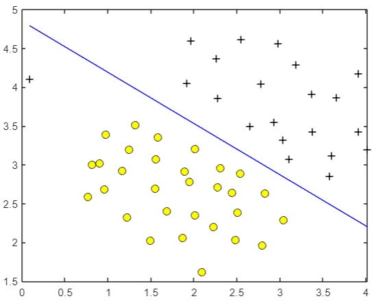
C = 1;
model = svmTrain(X, y, C, @linearKernel, 1e-3, 20);
visualizeBoundaryLinear(X, y, model);
The trained model is more reasonable. It does not forcibly include abnormal samples. At the same time, it is a large spacing model. The decision boundary is drawn in the center of the two categories, which is comfortable to look at.
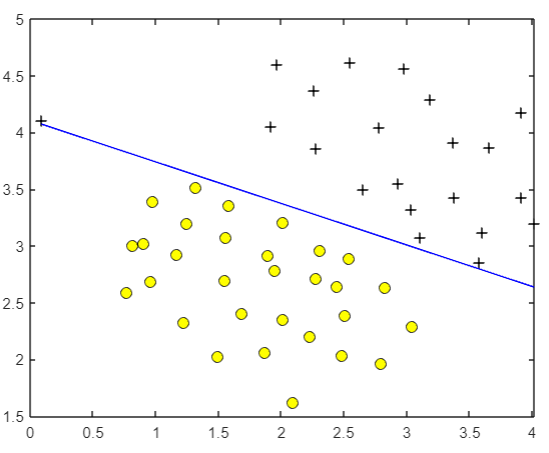
But if
C
C
When C is increased to 100, the fitting requirements of the algorithm for samples become very strict, so the model will try its best to include abnormal points, and look at the sub son that is not very good:
Complex nonlinear boundary
For the following data, it is obvious that a straight line cannot solve the problem:
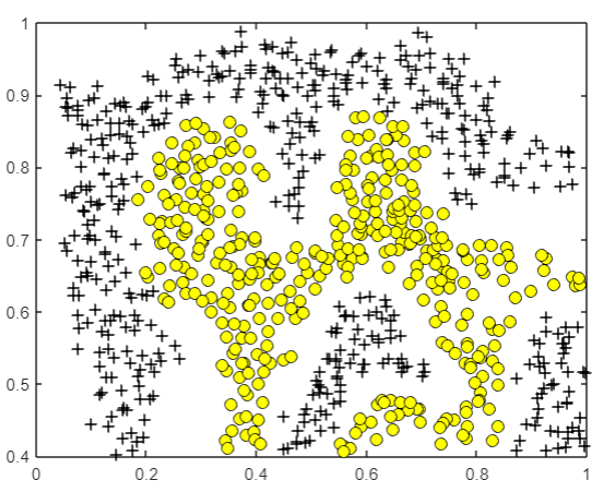
Therefore, we need to add kernel function to construct complex nonlinear boundary, and write Gaussian function as kernel function:
f
=
similarity
(
x
⃗
,
l
⃗
)
=
exp
(
−
∣
∣
x
⃗
−
l
⃗
∣
∣
2
2
σ
2
)
f=\text{similarity}(\vec{x},\vec{l})=\exp(-\frac{||\vec{x}-\vec{l}||^2}{2\sigma^2})
f=similarity(x
,l
)=exp(−2σ2∣∣x
−l
∣∣2)
function sim = gaussianKernel(x1, x2, sigma)
%RBFKERNEL returns a radial basis function kernel between x1 and x2
%   sim = gaussianKernel(x1, x2) returns a gaussian kernel between x1 and x2
%   and returns the value in sim

% Ensure that x1 and x2 are column vectors
x1 = x1(:); x2 = x2(:);

% You need to return the following variables correctly.
sim = 0;

% ====================== YOUR CODE HERE ======================
% Instructions: Fill in this function to return the similarity between x1
%               and x2 computed using a Gaussian kernel with bandwidth
%               sigma
%
%

sim=(x1-x2)'*(x1-x2);
sim=exp(-sim/(2*sigma^2));
% =============================================================

end
Then call the big guy's function and wait for the result:
% SVM Parameters
C = 1; sigma = 0.1;

% We set the tolerance and max_passes lower here so that the code will run faster. However, in practice,
% you will want to run the training to convergence.
model= svmTrain(X, y, C, @(x1, x2) gaussianKernel(x1, x2, sigma));
visualizeBoundary(X, y, model);

Parameter selection
In the previous question, parameters C C C and σ \sigma σ Wu Enda gave it to us. When we build our own model, we need to choose the parameters ourselves. This requires a program to help us enumerate parameters and train on the training set, and finally find the most appropriate parameters through the verification set:
function [C, sigma] = dataset3Params(X, y, Xval, yval)
%DATASET3PARAMS returns your choice of C and sigma for Part 3 of the exercise
%where you select the optimal (C, sigma) learning parameters to use for SVM
%with RBF kernel
%   [C, sigma] = DATASET3PARAMS(X, y, Xval, yval) returns your choice of C and
%   sigma. You should complete this function to return the optimal C and
%   sigma based on a cross-validation set.
%

C_vec = [0.01, 0.03, 0.1, 0.3, 1, 3, 10, 30];
sigma_vec = [0.01, 0.03, 0.1, 0.3, 1, 3, 10, 30];
n=length(C_vec);
m=length(sigma_vec);

% ====================== YOUR CODE HERE ======================
% Instructions: Fill in this function to return the optimal C and sigma
%               learning parameters found using the cross validation set.
%               You can use svmPredict to predict the labels on the cross
%               validation set. For example,
%                   predictions = svmPredict(model, Xval);
%               will return the predictions on the cross validation set.
%
%  Note: You can compute the prediction error using
%        mean(double(predictions ~= yval))
%
error=10^10;
for i=1:n
    for j=1:m
        C=C_vec(i);
        sigma=sigma_vec(j);%enumerated parameter
        model=svmTrain(X,y,C,@(x1,x2)gaussianKernel(x1, x2, sigma));
        predictions=svmPredict(model,Xval);%Train and predict
        if error>mean(double(predictions~=yval))%Calculate and update the minimum error
            error=mean(double(predictions~=yval));
            p=i;
            q=j;
        end
    end
end
C=C_vec(p);
sigma=sigma_vec(q);
% =========================================================================

end
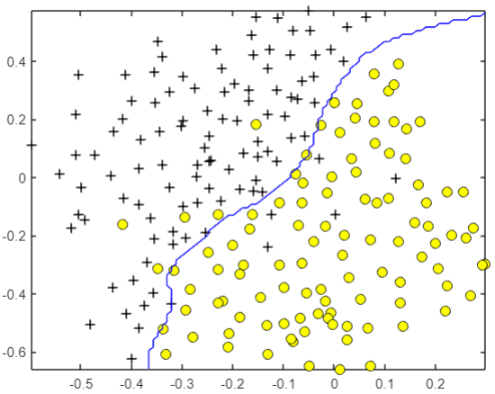
Finally, for the following data, we get the decision boundary as shown in the figure:
% Try different SVM Parameters here
[C, sigma] = dataset3Params(X, y, Xval, yval);

% Train the SVM
model = svmTrain(X, y, C, @(x1, x2)gaussianKernel(x1, x2, sigma));
visualizeBoundary(X, y, model);