catalogue
1. There is a problem with the original GAN
Reference article: Amazing Wasserstein GAN - Zhihu (zhihu.com)
1. There is a problem with the original GAN
In practical training, GAN has some problems, such as difficult training, the loss of generator and discriminator can not indicate the training process, the lack of diversity of generated samples and so on. This is related to the mechanism of GAN. The Nash equilibrium that GAN finally achieves confrontation is only an ideal state, while the results obtained in reality are intermediate states (pseudo equilibrium).
In most cases, the more training times, the better the effect of discriminator D, which will always distinguish the output of generator G from the real sample. This is because generator G maps from low-dimensional space to high-dimensional space (complex sample space), and the generated sample distribution space Pg is difficult to fill the distribution space Pr of the whole real sample. That is, the two distributions do not overlap at all, or their overlapping parts can be ignored, so that the discriminator D will always separate them.
In the training of the original GAN, if the discriminator is trained too well, the gradient of the generator will disappear and the loss of the generator will not be reduced; If the discriminator is not well trained, the gradient of the generator will be inaccurate and run around. Only the discriminator is trained to the best intermediate state, but this scale is difficult to grasp, and there is no basis for convergence judgment. Even in different stages before and after the same round of training, the time period of this state is different, which is completely uncontrollable.
Kullback Leibler divergence (KL divergence for short) and Jensen Shannon divergence (JS divergence for short) are introduced as two important similarity measurement indicators. Wasserstein distance, one of the later protagonists, is to sling them. So next, we will introduce these two important supporting roles - KL divergence and JS divergence:
According to the original discriminator of loss, we can get the optimal discriminator of loss; Under the optimal discriminator, we can transform the generator loss defined by the original GAN into minimizing the JS divergence between the real distribution and the generated distribution. The more we train the discriminator, the closer it will be to the optimum, and the loss of the minimization generator will be closer to the JS divergence between the minimization and.
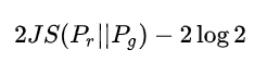
The first form of loss, whether it is far away or near, as long as there is no overlap or the overlap can be ignored, the JS divergence is fixed as a constant, which means for the gradient descent method - the gradient is 0! At this time, for the optimal discriminator, the generator must not get a little gradient information; Even for the near optimal discriminator, the generator has a great chance to face the problem of gradient disappearance.
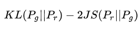
The second form of loss has two serious problems. The first is that it should minimize the KL divergence of generated distribution and real distribution at the same time, but maximize the JS divergence of both. One should be closer and the other should be pushed away! This is very absurd intuitively, but it will lead to gradient instability numerically. This is the problem of the later JS divergence term.
Summary of the first part: under the (approximate) optimal discriminator of the original GAN, the first generator loss faces the problem of gradient disappearance, and the second generator loss faces the problems of absurd optimization objectives, unstable gradient and unbalanced punishment for diversity and accuracy, resulting in mode collapse.
The origin of the original GAN problem can be attributed to two points: one is that the distance measurement of equivalent optimization (KL divergence and JS divergence) is unreasonable; the other is that the generated distribution after random initialization of the generator is difficult to overlap with the real distribution.
2 WGAN principle
WGan (Wasserstein Gan), Wasserstein refers to Wasserstein distance, also known as earth mover (EM) bulldozer distance, which is defined as follows:
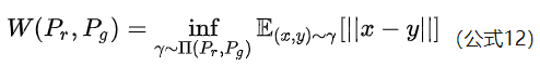
The advantage of Wasserstein distance over KL divergence and JS divergence is that even if the two distributions do not overlap, Wasserstein distance can still reflect their distance. WGAN shows this through simple examples. Consider the following two distribution sums in two-dimensional space, which are evenly distributed on line AB and CD. The distance between the two distributions can be controlled by controlling parameters.
WGan's idea is to combine the generated simulated sample distribution Pg with the original sample distribution Pr as a set of all possible joint distributions. Then the real sample and the simulated sample can be sampled, and the distance between them can be calculated, and the expected value of the distance can also be calculated.
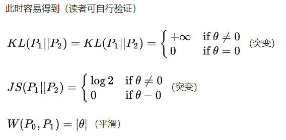
KL divergence and JS divergence are abrupt, either the largest or the smallest, but the Wasserstein distance is smooth. If we want to optimize this parameter by gradient descent method, the first two can not provide gradient at all, but the Wasserstein distance can. Similarly, in high-dimensional space, if the two distributions do not overlap or the overlapping part can be ignored, KL and JS can neither reflect the distance nor provide a gradient, but Wasserstein can provide a meaningful gradient.
When using W-GAN network for image generation, the network regards the whole image as an attribute, and its purpose is to learn the data distribution of the whole attribute of the image. Therefore, it is reasonable and feasible to fit the generated image distribution Pg to the real image distribution Pr. If the desired generation distribution Pg is not the current real image distribution Pr, the specific convergence direction of the network will be uncontrollable and the training will fail.
In this way, through training, the network can optimize the direction of taking the lower bound of the expected value in all possible joint distributions, that is, pull the set of two distributions together. In this way, the original discriminant is no longer the function of judging the authenticity, but the function of calculating the distance between two distribution sets. Therefore, it is more appropriate to call it a reviewer. Similarly, the sigmoid of the last layer needs to be removed.
Core idea: the loss of D of the original GAN is the cross entropy of the real sample and 1, and the cross entropy of the simulated sample and 0; The loss of G is the cross entropy of the simulated sample and 1. WGan's loss is to form a joint distribution of real samples and simulated samples, and make a difference between them after sampling. The purpose of D is that the larger the two, the better, and the purpose of G is that the smaller the two, the better.
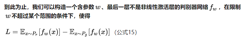
As far as possible, L will approximate the Wasserstein distance between the real distribution and the generated distribution (ignoring the constant multiple). Note that the discriminator of the original GAN does the true and false binary classification task, so the last layer is sigmoid, but now the discriminator in WGAN does the approximate fitting of Wasserstein distance, which belongs to the regression task, so the sigmoid of the last layer should be removed.
Next, the generator should approximately minimize the Wasserstein distance, which can minimize L. due to the excellent properties of the Wasserstein distance, we don't need to worry about the disappearance of the generator gradient. Considering that the first item is independent of the generator, we get two loss es of WGAN.
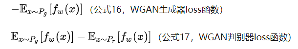
Formula 15 is the inverse of formula 17, which can indicate the training process. The smaller the value, the smaller the Wasserstein distance between the real distribution and the generated distribution, and the better the GAN training.
3 code understanding
Compared with the first form of the original GAN, WGAN has only changed four points:
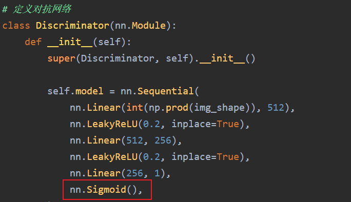
- The last layer of the discriminator removes sigmoid
- The loss of generator and discriminator does not take log
- Every time the parameters of the discriminator are updated, their absolute values are truncated to no more than a fixed constant c
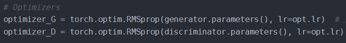
- Don't use momentum based optimization algorithms (including momentum and Adam), recommend RMSProp and SGD
For the modified part of GAN code, refer to the GAN code on the homepage for specific differences:
- Because it becomes a regression task, the Sigmoid function is removed.
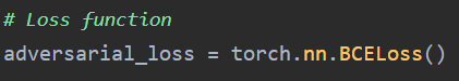
- Delete the Loss function.
- Instead of using momentum based optimization algorithms (including momentum and Adam), the optimizer is changed to RMSprop
- Guarantee f θ (x)f θ (x) Satisfying the K-Lipschitz condition, Wasserstein GAN makes a simple processing. Because the discriminator is composed of neural network, it can be realized by clamping the parameters in the linear operator of each layer and limiting its value range. As in this part of the code above. The clamp function is used to take the upper and lower limits
# Clip weights of discriminator
for p in discriminator.parameters():
    p.data.clamp_(-opt.clip_value, opt.clip_value)
- Modify the calculation method of loss:
loss_D = -torch.mean(discriminator(real_imgs)) + torch.mean(discriminator(fake_imgs))
loss_G = -torch.mean(discriminator(gen_imgs))
GitHub source code
import argparse
import os
import numpy as np
import math
import sys

import torchvision.transforms as transforms
from torchvision.utils import save_image

from torch.utils.data import DataLoader
from torchvision import datasets
from torch.autograd import Variable

import torch.nn as nn
import torch.nn.functional as F
import torch

os.makedirs("images", exist_ok=True)

parser = argparse.ArgumentParser()
parser.add_argument("--n_epochs", type=int, default=200, help="number of epochs of training")
parser.add_argument("--batch_size", type=int, default=64, help="size of the batches")
parser.add_argument("--lr", type=float, default=0.00005, help="learning rate")
parser.add_argument("--n_cpu", type=int, default=8, help="number of cpu threads to use during batch generation")
parser.add_argument("--latent_dim", type=int, default=100, help="dimensionality of the latent space")
parser.add_argument("--img_size", type=int, default=28, help="size of each image dimension")
parser.add_argument("--channels", type=int, default=1, help="number of image channels")
parser.add_argument("--n_critic", type=int, default=5, help="number of training steps for discriminator per iter")
parser.add_argument("--clip_value", type=float, default=0.01, help="lower and upper clip value for disc. weights")
parser.add_argument("--sample_interval", type=int, default=400, help="interval betwen image samples")
opt = parser.parse_args()
print(opt)

img_shape = (opt.channels, opt.img_size, opt.img_size)

cuda = True if torch.cuda.is_available() else False


class Generator(nn.Module):
    def __init__(self):
        super(Generator, self).__init__()

        def block(in_feat, out_feat, normalize=True):
            layers = [nn.Linear(in_feat, out_feat)]
            if normalize:
                layers.append(nn.BatchNorm1d(out_feat, 0.8))
            layers.append(nn.LeakyReLU(0.2, inplace=True))
            return layers

        self.model = nn.Sequential(
            *block(opt.latent_dim, 128, normalize=False),
            *block(128, 256),
            *block(256, 512),
            *block(512, 1024),
            nn.Linear(1024, int(np.prod(img_shape))),
            nn.Tanh()
        )

    def forward(self, z):
        img = self.model(z)
        img = img.view(img.shape[0], *img_shape)
        return img


class Discriminator(nn.Module):
    def __init__(self):
        super(Discriminator, self).__init__()

        self.model = nn.Sequential(
            nn.Linear(int(np.prod(img_shape)), 512),
            nn.LeakyReLU(0.2, inplace=True),
            nn.Linear(512, 256),
            nn.LeakyReLU(0.2, inplace=True),
            nn.Linear(256, 1),
        )

    def forward(self, img):
        img_flat = img.view(img.shape[0], -1)
        validity = self.model(img_flat)
        return validity


# Initialize generator and discriminator
generator = Generator()
discriminator = Discriminator()

if cuda:
    generator.cuda()
    discriminator.cuda()

# Configure data loader
os.makedirs("../../data/mnist", exist_ok=True)
dataloader = torch.utils.data.DataLoader(
    datasets.MNIST(
        "../../data/mnist",
        train=True,
        download=True,
        transform=transforms.Compose([transforms.ToTensor(), transforms.Normalize([0.5], [0.5])]),
    ),
    batch_size=opt.batch_size,
    shuffle=True,
)

# Optimizers
optimizer_G = torch.optim.RMSprop(generator.parameters(), lr=opt.lr)
optimizer_D = torch.optim.RMSprop(discriminator.parameters(), lr=opt.lr)

Tensor = torch.cuda.FloatTensor if cuda else torch.FloatTensor

# ----------
#  Training
# ----------

batches_done = 0
for epoch in range(opt.n_epochs):

    for i, (imgs, _) in enumerate(dataloader):

        # Configure input
        real_imgs = Variable(imgs.type(Tensor))

        # ---------------------
        #  Train Discriminator
        # ---------------------

        optimizer_D.zero_grad()

        # Sample noise as generator input
        z = Variable(Tensor(np.random.normal(0, 1, (imgs.shape[0], opt.latent_dim))))

        # Generate a batch of images
        fake_imgs = generator(z).detach()
        # Adversarial loss
        loss_D = -torch.mean(discriminator(real_imgs)) + torch.mean(discriminator(fake_imgs))

        loss_D.backward()
        optimizer_D.step()

        # Clip weights of discriminator
        for p in discriminator.parameters():
            p.data.clamp_(-opt.clip_value, opt.clip_value)

        # Train the generator every n_critic iterations
        if i % opt.n_critic == 0:

            # -----------------
            #  Train Generator
            # -----------------

            optimizer_G.zero_grad()

            # Generate a batch of images
            gen_imgs = generator(z)
            # Adversarial loss
            loss_G = -torch.mean(discriminator(gen_imgs))

            loss_G.backward()
            optimizer_G.step()

            print(
                "[Epoch %d/%d] [Batch %d/%d] [D loss: %f] [G loss: %f]"
                % (epoch, opt.n_epochs, batches_done % len(dataloader), len(dataloader), loss_D.item(), loss_G.item())
            )

        if batches_done % opt.sample_interval == 0:
            save_image(gen_imgs.data[:25], "images/%d.png" % batches_done, nrow=5, normalize=True)
        batches_done += 1