catalogue
Unsupervised learning 1 -- clustering
What is unsupervised learning?
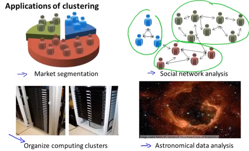
What are the applications of clustering?
Pseudo code represents the process of k-means
It is often used to solve the problem of poorly separated clusters
How to make the algorithm avoid local optimal solution?
Unsupervised learning 2 -- dimension reduction
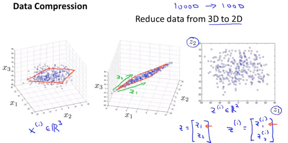
Objective 1 --- data compression
PCA (also called principal component analysis)
Principal component analysis problem planning 1
Formula description of PCA problem
Principal component analysis problem planning 2
Principal component fraction selection
1. A simple two-dimensional data set
2. Applied to image compression
1. Apply PCA to a simple two-dimensional data set
Unsupervised learning 1 -- clustering
What is unsupervised learning?
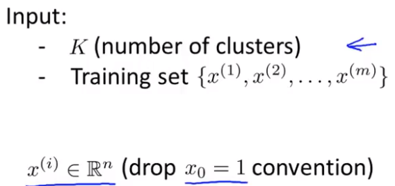
The training set has only x1, x2...,xi and no data labeled y.
We need to input unlabeled data, and then let the algorithm find some structures hidden in the data,
The clustering algorithm (the first unsupervised learning algorithm) divides these unlabeled data into clusters.
What are the applications of clustering?
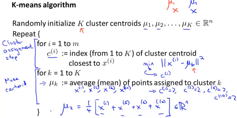
K-means algorithm
Language expression steps
Given a set of unlabeled data sets, it is hoped that an algorithm can automatically divide these data into closely related subsets or clusters.
K-means algorithm is one of the popular and widely used algorithms.
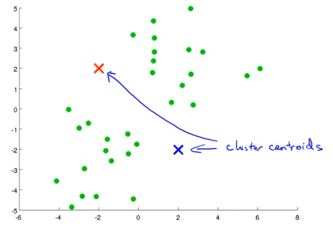
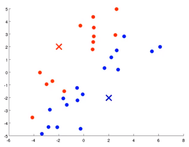
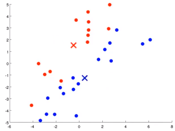
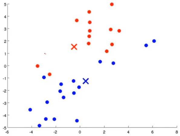
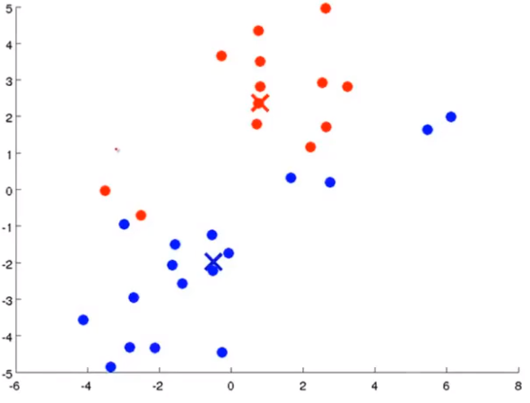
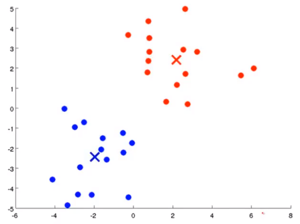
K-mean step: suppose I want to divide the data into two clusters
Firstly, two points are randomly generated, which are called cluster centers. K-means is an iterative algorithm that does two things: the first cluster allocation and the second mobile cluster center. Cluster classification: you need to traverse each data, and assign this data to that point according to the distance between it and two random points. Moving cluster center: find all points of the same color and calculate the position of their mean value as the new cluster center. Then calculate the distance between each point and the center point again, and repeat these two steps until the center point does not change.
Pseudo code represents the process of k-means
Note: suppose uk is the mean value of a cluster. If there is a cluster center without points, directly remove the cluster center and finally get K-1 clusters; If you want to the final K clusters, you need to reinitialize the cluster center; But the most common practice is to remove it directly.
It is often used to solve the problem of poorly separated clusters
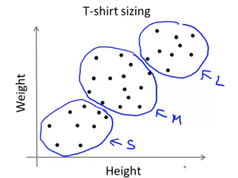 For example, the size of clothes will be designed according to their weight (S,L,M)
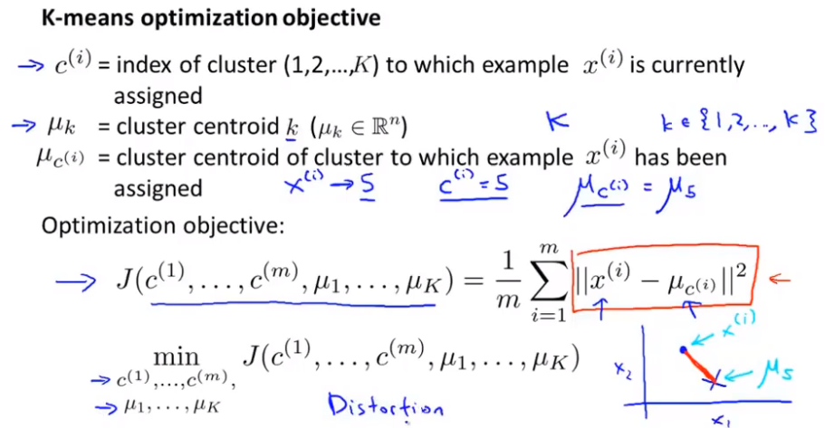
Optimization objectives
K: Indicates the number of clusters; k: Subscript indicating the cluster center point, c^i: indicating the cluster into which xi is divided.
The cost function of K-means is j in the figure below. The algorithm finally needs to find c^i, μ_ i. That is, the parameter value of J can be minimized. This cost function is sometimes called distortion cost function or K-means distortion. J - > distortion function
Random initialization
How to make the algorithm avoid local optimal solution?
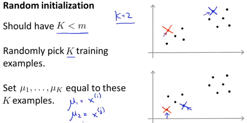 Different initialization points lead to different results.
Initializing the selected points may cause the results to fall into local optimization, as shown in the two figures in the lower right corner of the figure below.
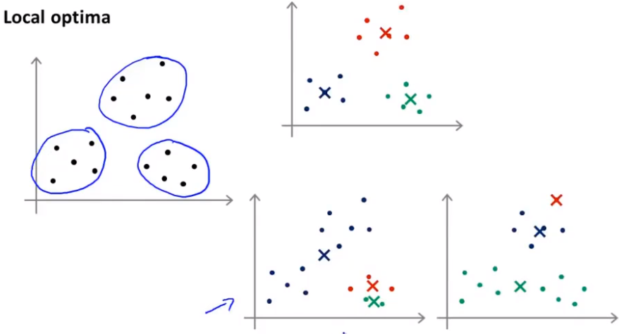
To avoid falling into local optimization, we need to initialize multiple times instead of once. To ensure that the final result is optimal.
The common initialization times are 50 to 1000. Of course, if K is small, the number of times is less.
Select the number of clusters
At present, there is no algorithm that can automatically select the number of clusters, which needs to be selected through visual data or observing the output of clusters (manual)
"Elbow rule"
If you get the curve of the left graph, it's good, but usually the graph you get is the right graph. You can't judge that point, so it's equivalent to doing nothing.
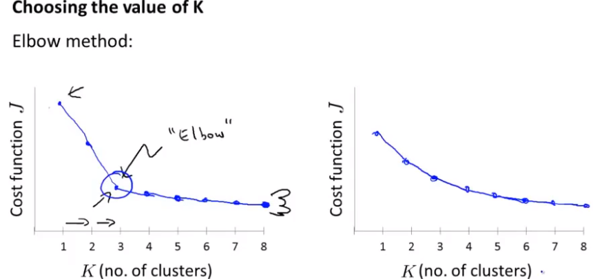 So don't expect it to work every time.
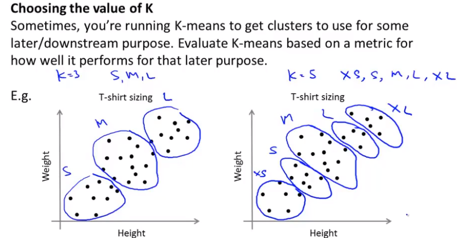
The following still takes clothing size clustering as an example:
The sales volume of clothes may help you decide how to divide into several categories. How to use the follow-up purpose to decide what kind of clothes to use as the evaluation criteria to select the cluster number. When selecting manually, what is the purpose of clustering?
Unsupervised learning 2 -- dimension reduction
Objective 1 --- data compression
Compression can reduce the occupied space and make the learning algorithm run faster.
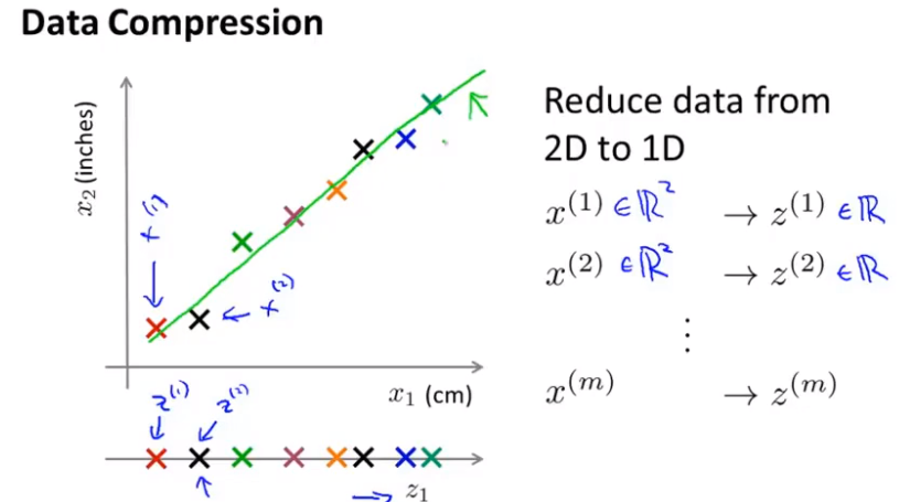
Figure 1 -- > Figure 2 (projecting data onto a plane) - > finally, it is reduced to two-dimensional space representation
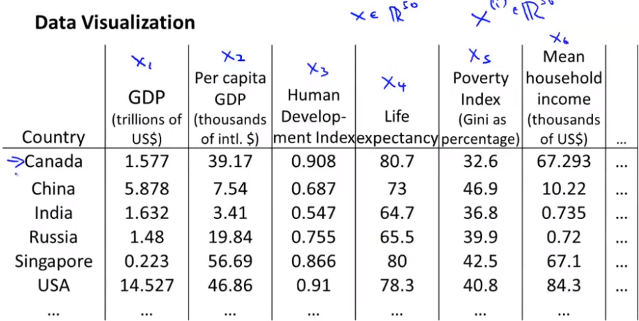
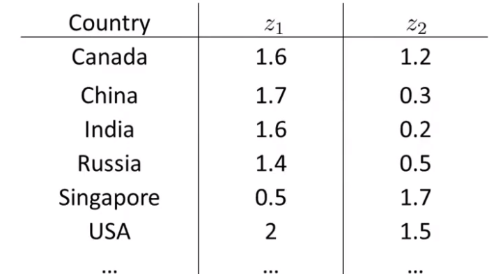
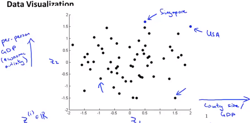
Objective 2 - visualization
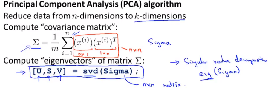
PCA (also called principal component analysis)
Principal component analysis problem planning 1
Formula description of PCA problem
Formula description is to use formula to describe the purpose of PCA. Principal component analysis
Mathematical proof is too complicated, so there is no mathematical proof here. Why can u and z be used like this.
As shown in the following figure: for a two-dimensional data, we want to find a straight line, project the point onto the straight line, it will find a low-dimensional plane (here is a straight line), and project the point onto the plane. The distance between each point and the projection is called "projection error". PCA will select the plane or line with the least square error as the projection plane or line, so as to minimize the plane projection error. 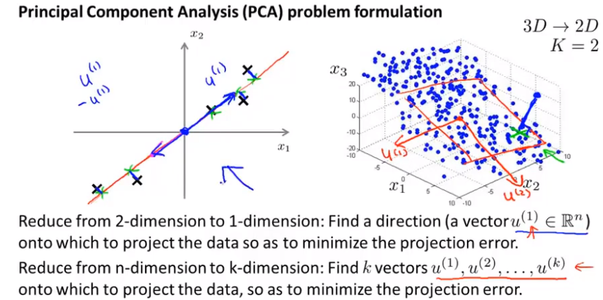
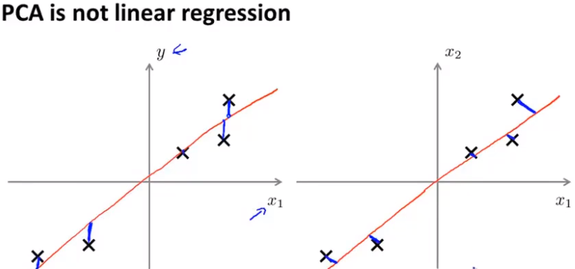
PCA and linear regression
Firstly, PCA is not linear regression, they are two different algorithms, and their calculation errors are different, as shown in the figure below.
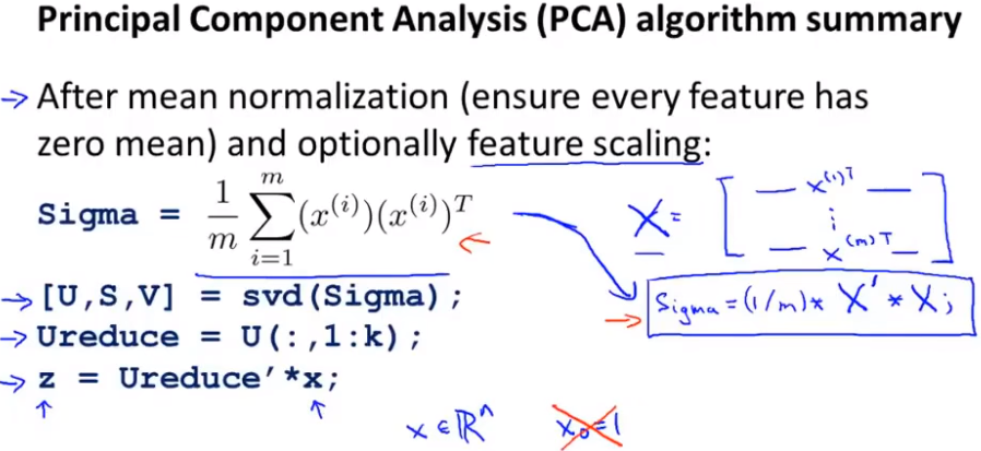
Principal component analysis problem planning 2
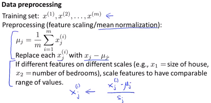
data processing
In unsupervised learning, the mean normalization process (making each feature have a mean of 0) is very similar to the feature scaling process (determined according to the data set).
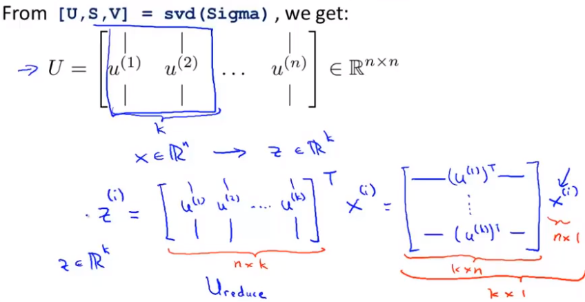
The description process of calculating u ^ (I) and Z is shown in the following figure, and the covariance is in Σ (in words) σ: A covariance matrix) indicates that the left side of the formula is covariance and the right side is summation symbol. svd: represents singular value decomposition. Just find a library with this function in different languages.
summary
After mean normalization, in order to ensure that each feature has a mean of 0. Scale optional features according to the data range. After preprocessing, calculate the carrier matrix Sigma. Through this method, if your data is given as a matrix, as shown in the X training set matrix in the figure, then we first get the first k columns of the dimension reduction matrix U, z =.. which defines how we go from an eigenvector x to the dimension reduction table Z.
Principal component fraction selection
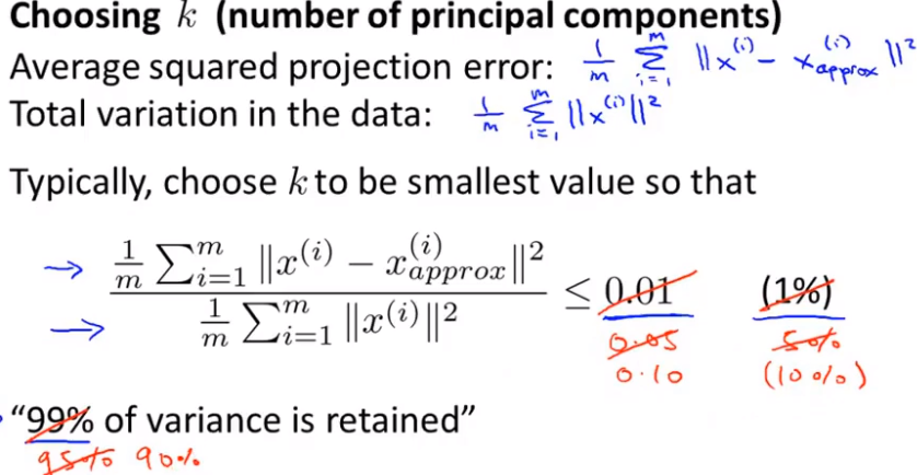
We hope to choose as small as possible when the ratio of mean square error to training set variance is as small as possible k value (from n features to k features). If we want this ratio to be less than 1%, it means that 99% of the deviation of the original data is retained. If we choose to retain 90% of the deviation, we can significantly reduce the dimension of features in the model.
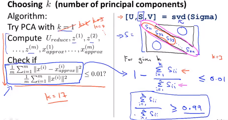 We can take shilling k=1 and then do principal component analysis to get U_{reduce}Ureduce} and z, and then calculate whether the proportion is less than 1%. If not, let k=2, and so on, until the minimum K value that can make the proportion less than 1% is found (because there is usually some correlation between various features) S is an n × n The matrix of has only values on the diagonal, while other cells are 0. We can use this matrix to calculate the ratio of the average mean square error to the variance of the training set:
Namely:

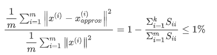
Compression reproduction
Reproduction, that is, how to get the previous data representation from the compressed data?
Suggestions for applying PCA
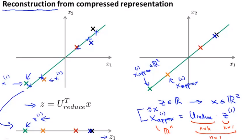
First, let's try using PCA to accelerate unsupervised learning algorithm. Suppose you have a supervised learning data, in which x^i has a high dimension. In practice, this may be a problem of computer vision. That is, suppose we have a 100 × A 100 pixel picture contains 10000 pixel intensity values. For this high-dimensional feature vector, the learning algorithm is very slow. This is to reduce its dimension with PCA. The steps are as follows:
-
First, extract x without looking at y; use PCA to compress the data to 1000 features
-
Then, a learning algorithm is run on the training set: logistic regression, SVM, neural network, etc
-
Finally, if there is a new sample, map the new test sample x through the mapping relationship of PAC to obtain the corresponding z, and then bring z to the hypothesis function
-
note:PCA defines a mapping from x to z, which can only be defined by running PCA on the training set. What it does is calculate a series of parameters for feature scaling and mean normalization, and it also calculates the matrix u_reduce (which can only be obtained from the training set)
 Incorrect use of PCA:
 -
It is considered that PCA is a method to prevent over fitting. The best way to prevent over fitting is regularization. The reason is that PCA only approximately discards some features, and it does not consider any influence related to y, so it may lose very important features.
-
By default, PCA is used as a part of the learning process. Although it is effective in many cases, it is recommended to start with all the original features before using PCA, and consider using PCA only when you are sure that x cannot run (the algorithm runs too slowly or occupies too much memory).
-
Total: PCA is used to improve algorithm efficiency, data compression and visualization.
K-means application ex7
1. A simple two-dimensional data set
import numpy as np
import pandas as pd
import matplotlib.pyplot as plt
import seaborn as sb
from scipy.io import loadmat

def find_closest_centroids(X, centroids):
    m = X.shape[0]
    k = centroids.shape[0]
    idx = np.zeros(m)

    for i in range(m):
        min_dist = 1000000
        for j in range(k):
            dist = np.sum((X[i,:] - centroids[j,:]) ** 2)
            if dist < min_dist:
                min_dist = dist
                idx[i] = j

    return idx

data = loadmat('E:/Python/machine learning/data/ex7data2.mat')
X = data['X']
initial_centroids = initial_centroids = np.array([[3, 3], [6, 2], [8, 5]])

idx = find_closest_centroids(X, initial_centroids)
idx[0:3]
array([0., 2., 1.])
data2 = pd.DataFrame(data.get('X'), columns=['X1', 'X2'])
data2.head()| X1 | X2 | |
|---|---|---|
| 0 | 1.842080 | 4.607572 |
| 1 | 5.658583 | 4.799964 |
| 2 | 6.352579 | 3.290854 |
| 3 | 2.904017 | 4.612204 |
| 4 | 3.231979 | 4.939894 |
#Data visualization
sb.set(context="notebook", style="white")
sb.lmplot('X1', 'X2', data=data2, fit_reg=False)
plt.show()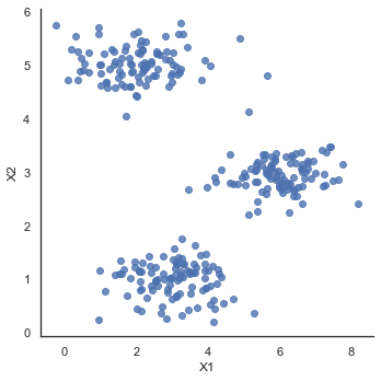
def compute_centroids(X, idx, k):
    m, n = X.shape
    centroids = np.zeros((k, n))

    for i in range(k):
        indices = np.where(idx == i)
        centroids[i,:] = (np.sum(X[indices,:], axis=1) / len(indices[0])).ravel()

    return centroids

compute_centroids(X, idx, 3)
array([[1.95399466, 5.02557006],
[3.04367119, 1.01541041],
[6.03366736, 3.00052511]])
# Assign the sample to the nearest cluster and recalculate the cluster center of the cluster
def run_k_means(X, initial_centroids, max_iters):
    m, n = X.shape
    k = initial_centroids.shape[0]
    idx = np.zeros(m)
    centroids = initial_centroids

    for i in range(max_iters):
        idx = find_closest_centroids(X, centroids)
        centroids = compute_centroids(X, idx, k)

    return idx, centroids

idx, centroids = run_k_means(X, initial_centroids, 10)

cluster1 = X[np.where(idx == 0)[0],:]
cluster2 = X[np.where(idx == 1)[0],:]
cluster3 = X[np.where(idx == 2)[0],:]

fig, ax = plt.subplots(figsize=(12,8))
ax.scatter(cluster1[:,0], cluster1[:,1], s=30, color='r', label='Cluster 1')
ax.scatter(cluster2[:,0], cluster2[:,1], s=30, color='g', label='Cluster 2')
ax.scatter(cluster3[:,0], cluster3[:,1], s=30, color='b', label='Cluster 3')
ax.legend()
plt.show()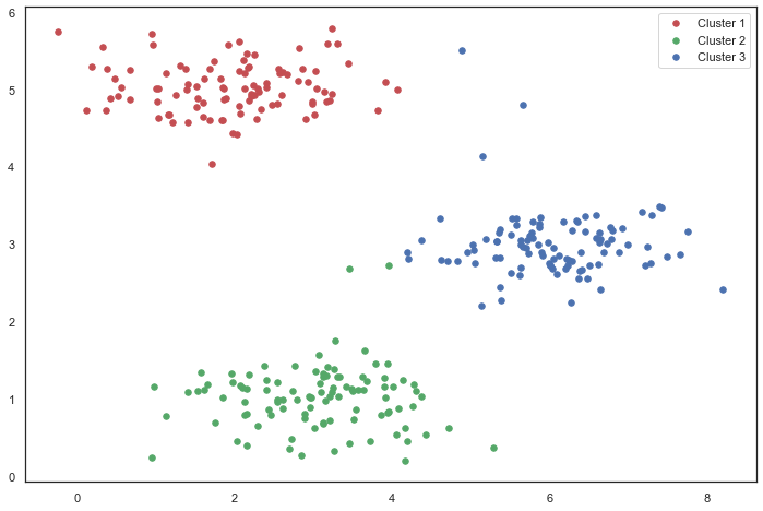
# Create a function that selects a random sample and uses it as the initial cluster center

def init_centroids(X, k):
    m, n = X.shape
    centroids = np.zeros((k, n))
    idx = np.random.randint(0, m, k)

    for i in range(k):
        centroids[i,:] = X[idx[i],:]

    return centroids

init_centroids(X, 3)
array([[3.18412176, 1.41410799],
[1.30882588, 5.30158701],
[1.95538864, 1.32156857]])
2. Applied to image compression
Here, you need to turn to skimage secretly, but an error will be reported when you install it directly. You need to PIP install scikit image first. This needs to wait a while before pip install skimage. There is a problem with my installation. Woo woo woo
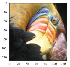
from IPython.display import Image
Image(filename='E:/Python/machine learning/data/bird_small.png')

# Original pixel measured pixel value
image_data = loadmat('E:/Python/machine learning/data/bird_small.mat')
image_data
{'__header__': b'MATLAB 5.0 MAT-file, Platform: GLNXA64, Created on: Tue Jun 5 04:06:24 2012',
'__version__': '1.0',
'__globals__': [],
'A': array([[[219, 180, 103],
[230, 185, 116],
[226, 186, 110],
...,
[ 14, 15, 13],
[ 13, 15, 12],
[ 12, 14, 12]],
[[230, 193, 119],
[224, 192, 120],
[226, 192, 124],
...,
[ 16, 16, 13],
[ 14, 15, 10],
[ 11, 14, 9]],
[[228, 191, 123],
[228, 191, 121],
[220, 185, 118],
...,
[ 14, 16, 13],
[ 13, 13, 11],
[ 11, 15, 10]],
...,
[[ 15, 18, 16],
[ 18, 21, 18],
[ 18, 19, 16],
...,
[ 81, 45, 45],
[ 70, 43, 35],
[ 72, 51, 43]],
[[ 16, 17, 17],
[ 17, 18, 19],
[ 20, 19, 20],
...,
[ 80, 38, 40],
[ 68, 39, 40],
[ 59, 43, 42]],
[[ 15, 19, 19],
[ 20, 20, 18],
[ 18, 19, 17],
...,
[ 65, 43, 39],
[ 58, 37, 38],
[ 52, 39, 34]]], dtype=uint8)}
A = image_data['A']
A.shape
(128, 128, 3)
# Apply some preprocessing to the data and provide it to the K-means algorithm

# normalize value ranges
A = A / 255.

# reshape the array
X = np.reshape(A, (A.shape[0] * A.shape[1], A.shape[2]))
print(X.shape)

# randomly initialize the centroids
initial_centroids = init_centroids(X, 16)

# run the algorithm
idx, centroids = run_k_means(X, initial_centroids, 10)

# get the closest centroids one last time
idx = find_closest_centroids(X, centroids)

# map each pixel to the centroid value
X_recovered = centroids[idx.astype(int),:]
print(X_recovered.shape)

# reshape to the original dimensions
X_recovered = np.reshape(X_recovered, (A.shape[0], A.shape[1], A.shape[2]))
print(X_recovered.shape)
(16384, 3)
(16384, 3)
(128, 128, 3)
plt.imshow(X_recovered)
plt.show()
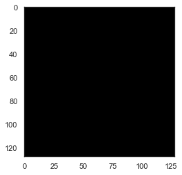 I don't know why it's black when I run it
Normal should be as follows:
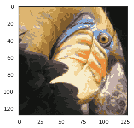
# We can see that we have compressed the image, but the main features of the image still exist
# This is K-means. Let's use scikit learn to implement K-means
from skimage import io
# cast to float, you need to do this otherwise the color would be weird after clustring
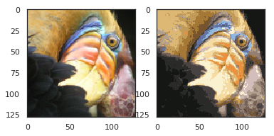
pic = io.imread('E:/Python/machine learning/data/bird_small.png') / 255.
io.imshow(pic)
plt.show()
print(pic.shape)

# serialize data
data = pic.reshape(128*128, 3)

print(data.shape)

from sklearn.cluster import KMeans#Import kmeans Library

model = KMeans(n_clusters=16, n_init=100, n_jobs=-1)

model.fit(data)
(128, 128, 3)
(16384, 3)
KMeans(algorithm='auto', copy_x=True, init='k-means++', max_iter=300,
    n_clusters=16, n_init=100, n_jobs=-1, precompute_distances='auto',
    random_state=None, tol=0.0001, verbose=0)
centroids = model.cluster_centers_
print(centroids.shape)

C = model.predict(data)
print(C.shape)

print(centroids[C].shape)

compressed_pic = centroids[C].reshape((128,128,3))

fig, ax = plt.subplots(1, 2)
ax[0].imshow(pic)
ax[1].imshow(compressed_pic)
plt.show()
PCAex7
1. Apply PCA to a simple two-dimensional data set
# PCA1
data = loadmat('E:/Python/machine learning/data/ex7data1.mat')
data
{'__header__': b'MATLAB 5.0 MAT-file, Platform: PCWIN64, Created on: Mon Nov 14 22:41:44 2011',
'__version__': '1.0',
'__globals__': [],
'X': array([[3.38156267, 3.38911268],
[4.52787538, 5.8541781 ],
[2.65568187, 4.41199472],
[2.76523467, 3.71541365],
[2.84656011, 4.17550645],
[3.89067196, 6.48838087],
[3.47580524, 3.63284876],
[5.91129845, 6.68076853],
[3.92889397, 5.09844661],
[4.56183537, 5.62329929],
[4.57407171, 5.39765069],
[4.37173356, 5.46116549],
[4.19169388, 4.95469359],
[5.24408518, 4.66148767],
[2.8358402 , 3.76801716],
[5.63526969, 6.31211438],
[4.68632968, 5.6652411 ],
[2.85051337, 4.62645627],
[5.1101573 , 7.36319662],
[5.18256377, 4.64650909],
[5.70732809, 6.68103995],
[3.57968458, 4.80278074],
[5.63937773, 6.12043594],
[4.26346851, 4.68942896],
[2.53651693, 3.88449078],
[3.22382902, 4.94255585],
[4.92948801, 5.95501971],
[5.79295774, 5.10839305],
[2.81684824, 4.81895769],
[3.88882414, 5.10036564],
[3.34323419, 5.89301345],
[5.87973414, 5.52141664],
[3.10391912, 3.85710242],
[5.33150572, 4.68074235],
[3.37542687, 4.56537852],
[4.77667888, 6.25435039],
[2.6757463 , 3.73096988],
[5.50027665, 5.67948113],
[1.79709714, 3.24753885],
[4.3225147 , 5.11110472],
[4.42100445, 6.02563978],
[3.17929886, 4.43686032],
[3.03354125, 3.97879278],
[4.6093482 , 5.879792 ],
[2.96378859, 3.30024835],
[3.97176248, 5.40773735],
[1.18023321, 2.87869409],
[1.91895045, 5.07107848],
[3.95524687, 4.5053271 ],
[5.11795499, 6.08507386]])}
X = data['X']

fig, ax = plt.subplots(figsize=(12,8))
ax.scatter(X[:, 0], X[:, 1])
plt.show()
# The PCA algorithm is quite simple. After ensuring that the data is normalized, the output is only the singular value decomposition of the covariance matrix of the original data
def pca(X):
    # normalize the features
    X = (X - X.mean()) / X.std()

    # compute the covariance matrix
    X = np.matrix(X)
    cov = (X.T * X) / X.shape[0]

    # perform SVD
    U, S, V = np.linalg.svd(cov)

    return U, S, V

U, S, V = pca(X)
U, S, V
(matrix([[-0.79241747, -0.60997914],
[-0.60997914, 0.79241747]]),
array([1.43584536, 0.56415464]),
matrix([[-0.79241747, -0.60997914],
[-0.60997914, 0.79241747]]))
# A function that calculates the projection and selects only the top K components is implemented, which effectively reduces the dimension
def project_data(X, U, k):
    U_reduced = U[:,:k]
    return np.dot(X, U_reduced)

Z = project_data(X, U, 1)
Z
matrix([[-4.74689738],
        [-7.15889408],
        [-4.79563345],
        [-4.45754509],
        [-4.80263579],
        [-7.04081342],
        [-4.97025076],
        [-8.75934561],
        [-6.2232703 ],
        [-7.04497331],
        [-6.91702866],
        [-6.79543508],
        [-6.3438312 ],
        [-6.99891495],
        [-4.54558119],
        [-8.31574426],
        [-7.16920841],
        [-5.08083842],
        [-8.54077427],
        [-6.94102769],
        [-8.5978815 ],
        [-5.76620067],
        [-8.2020797 ],
        [-6.23890078],
        [-4.37943868],
        [-5.56947441],
        [-7.53865023],
        [-7.70645413],
        [-5.17158343],
        [-6.19268884],
        [-6.24385246],
        [-8.02715303],
        [-4.81235176],
        [-7.07993347],
        [-5.45953289],
        [-7.60014707],
        [-4.39612191],
        [-7.82288033],
        [-3.40498213],
        [-6.54290343],
        [-7.17879573],
        [-5.22572421],
        [-4.83081168],
        [-7.23907851],
        [-4.36164051],
        [-6.44590096],
        [-2.69118076],
        [-4.61386195],
        [-5.88236227],
        [-7.76732508]])
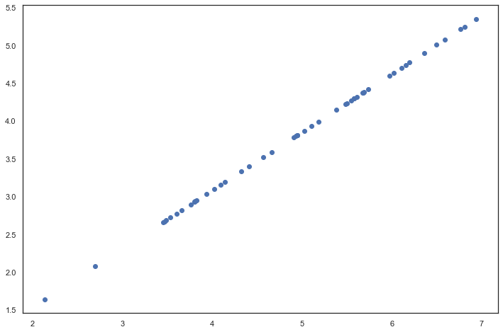
# We can also restore the original data through the reverse conversion step.
def recover_data(Z, U, k):
    U_reduced = U[:,:k]
    return np.dot(Z, U_reduced.T)

X_recovered = recover_data(Z, U, 1)
X_recovered
matrix([[3.76152442, 2.89550838],
[5.67283275, 4.36677606],
[3.80014373, 2.92523637],
[3.53223661, 2.71900952],
[3.80569251, 2.92950765],
[5.57926356, 4.29474931],
[3.93851354, 3.03174929],
[6.94105849, 5.3430181 ],
[4.93142811, 3.79606507],
[5.58255993, 4.29728676],
[5.48117436, 4.21924319],
[5.38482148, 4.14507365],
[5.02696267, 3.8696047 ],
[5.54606249, 4.26919213],
[3.60199795, 2.77270971],
[6.58954104, 5.07243054],
[5.681006 , 4.37306758],
[4.02614513, 3.09920545],
[6.76785875, 5.20969415],
[5.50019161, 4.2338821 ],
[6.81311151, 5.24452836],
[4.56923815, 3.51726213],
[6.49947125, 5.00309752],
[4.94381398, 3.80559934],
[3.47034372, 2.67136624],
[4.41334883, 3.39726321],
[5.97375815, 4.59841938],
[6.10672889, 4.70077626],
[4.09805306, 3.15455801],
[4.90719483, 3.77741101],
[4.94773778, 3.80861976],
[6.36085631, 4.8963959 ],
[3.81339161, 2.93543419],
[5.61026298, 4.31861173],
[4.32622924, 3.33020118],
[6.02248932, 4.63593118],
[3.48356381, 2.68154267],
[6.19898705, 4.77179382],
[2.69816733, 2.07696807],
[5.18471099, 3.99103461],
[5.68860316, 4.37891565],
[4.14095516, 3.18758276],
[3.82801958, 2.94669436],
[5.73637229, 4.41568689],
[3.45624014, 2.66050973],
[5.10784454, 3.93186513],
[2.13253865, 1.64156413],
[3.65610482, 2.81435955],
[4.66128664, 3.58811828],
[6.1549641 , 4.73790627]])
fig, ax = plt.subplots(figsize=(12,8))
ax.scatter(list(X_recovered[:, 0]), list(X_recovered[:, 1]))
plt.show()
# Note that the projection axis of the first principal component is basically the diagonal in the data set. When we reduce the data to one dimension, we lose the changes around the diagonal,
# So in our reproduction, everything goes along the diagonal
2. Apply PCA to face image
faces = loadmat('E:/Python/machine learning/data/ex7faces.mat')
X = faces['X']
X.shape
(5000, 1024)
def plot_n_image(X, n):
""" plot first n images
n has to be a square number
"""
pic_size = int(np.sqrt(X.shape[1]))
grid_size = int(np.sqrt(n))
first_n_images = X[:n, :]
fig, ax_array = plt.subplots(nrows=grid_size, ncols=grid_size,
sharey=True, sharex=True, figsize=(8, 8))
for r in range(grid_size):
for c in range(grid_size):
ax_array[r, c].imshow(first_n_images[grid_size * r + c].reshape((pic_size, pic_size)))
plt.xticks(np.array([]))
plt.yticks(np.array([]))
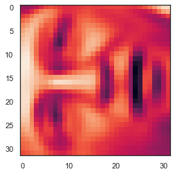
face = np.reshape(X[3,:], (32, 32))
plt.imshow(face)
plt.show()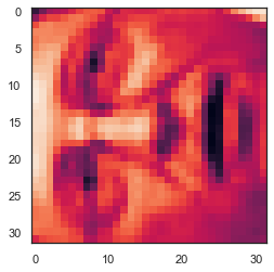
# It looks terrible. These images are only 32 x 32 grayscale (it is also a side rendering, but we can ignore it now). Our next step is to run PCA on the face dataset and get the first 100 main features.

U, S, V = pca(X)
Z = project_data(X, U, 100)

# Now we can try to restore the original structure and render again.
X_recovered = recover_data(Z, U, 100)
face = np.reshape(X_recovered[3,:], (32, 32))
plt.imshow(face)
plt.show()
# Note that we lost some details, although we didn't reduce the number of dimensions by 10 times as you expected