1. Introduction of attention mechanism

In the seq2seq model in the previous section, in order to enable the decoder and the linear classification layer to directly obtain more information during decoding, we provide the original context vector to each decoder and the original context vector and word embedding to each linear layer, as shown below:

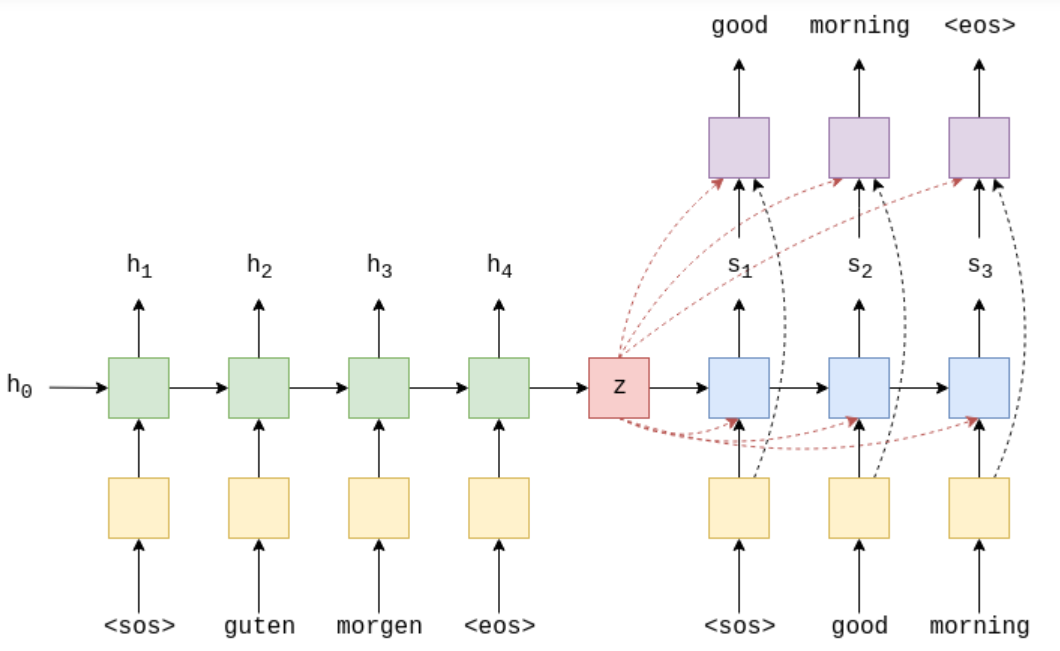
But it still can't change an essential place. The context vector is over compressed. That is, after multiple time steps of encoder compression, the smaller the previous information is retained, the less. When the decoder translates, it obtains little previous information, which further leads to the decline of model quality. Northern machine translation by joint learning to align and translate puts forward the attention mechanism, which improves the original context vector input by each encoder and linear layer. The so-called context vector is no longer the dense vector compressed by the encoder, but performs a "match" calculation between the output of each encoder and the hidden state of the current decoder input, calculates a "match" score for the output of each encoder, and then converts all the match scores into their weight probability through softmax calculation, The weight probability is weighted and summed with the corresponding encoder output to obtain the context vector. The model is as follows:

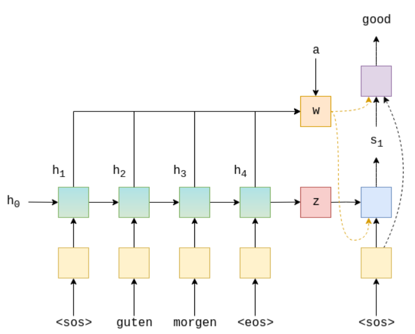
Firstly, the hidden state of s1 input is the original context vector z (s_t-1 for the later decoder). z is "matched" with the output [h1,h2,h3,h4] of each encoder (there are many calculation methods), and a matching score [score1,score2,score3,score4] is obtained. We transform it into the form of weight, that is, the matching score is calculated by softmax to obtain the weight matrix a[a1,a2,a3,a4]. Then calculate the context vector w=a1*h1+a2h2+a3h3+a4h4 corresponding to the current encoder. The advantages of this attention derived context vector are: (1) it has not been compressed too much, which reduces the loss of information. The previously input context vector is the last output of the encoder. Multiple encoding by the encoder causes the loss of previous useful information, while the attention vector is that each encoder output directly participates in the calculation of the last context vector. The loss of each encoder information is carried out according to the actual needs of the decoder. (2) Each decoder has its own attention weight matrix, because the hidden state of each decoder input is different, and the weight matrix is also different. For example, when we decode the first word, the probability of useful information is related to the output of the first encoder. The previous original context vector retains little information about the first encoder, while the attention vector can decide which encoder to prefer through its weight matrix (the closer the weight is to 1, the more it is retained. The closer it is to 0, the less it is retained).

In addition, considering that LSTM prefers the latest encoder, we used the method of reverse order before. Here is another new skill: bidirectional LSTM, as shown below:

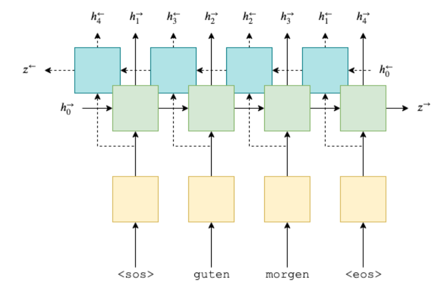
The positive LSTM is biased towards the second half of the sentence, while the reverse LSTM is biased towards the first half of the sentence. The two outputs are spliced to obtain the final output of bidirectional LSTM. Remember that the bidirectional LSTM is not a double layer, but can be understood as two independent lstms. One inputs the sentence from left to right, and the other inputs the sentence from right to left. Finally, the output of the two is spliced to obtain the final output, so the dimension of the output becomes twice that of the original. The hidden state output by the last encoder can be directly used as the original context vector before (assuming that the hidden state of the encoder and decoder is a dimension), but it is not possible now. The hidden state output by the last encoder is reduced to the decoded dimension through a linear layer and passes through a tanh activation function.

2. Calculation method of attention mechanism

Here, the attention mechanism is introduced according to the general situation:

The basic process of attention mechanism: for a sentence sequence, which consists of a sequence of wordsComposition.

(1) Applying some method willEach word inEncoded as a unique vector

(2) When decoding, the learned attention weight is usedWeighted linear combination of all vectors obtained in 1

(3) When the decoder predicts the next word, the linear combination obtained in (2) is used.

 

The specific core explanation of attention is as follows:

Our ultimate goal is to help the decoder have a weight reference for different words when generating words. During training, we have a training goal for the coder (i.e. we prefer a certain encoder). At this time, the information in the coder is defined as a Query (learning goal). The encoder contains all possible words. We regard it as a dictionary. The key of the dictionary is the sequence information of all encoders. N words are equivalent to n records in the current dictionary, and the value of the dictionary is usually the sequence information of all encoders. (in general, KV is equal) the next step is to calculate the weight of attention. Because we want the model to learn by itself, we should focus on those morphemes. Therefore, we need to use the learning target Query to participate in this process. Therefore, for each vector of Query, a function is used to calculate the weight of attention when predicting time t. Since the length of the encoder sequence is n, it should be an n-dimensional vector. Since the sum of weights is 1, the vector needs to be softmax normalized so that each one-dimensional element of the vector is a probability value.

 

Weight calculation method:

(1) Multilayer perceptron method (common)

It is mainly to splice the query and key, then connect a full connection of the activation function tanh (this is the end of this article), and then multiply it with the weight matrix defined by a network. This method is said to be particularly effective for large-scale data.

(2) Bilinear method

The mapping relationship between q and k is directly established in a sentence, which is more direct and faster.

 

(3)Dot Product

This method is more direct, saves the weight matrix, and directly establishes the relationship mapping between q and k. The advantage is that the calculation speed is faster, no parameters are required, and the complexity of the model is reduced. But the dimensions of q and k should be the same.

 

(4) Scaled dot product (commonly used, and self attention is also used)

One problem with the above dot product method is that with the increase of vector dimension, the final calculated score will be very large. After softmax is changed, the gradient will be very small (close to 0) during reverse derivation such as softmax calculation during back propagation. Therefore, normalize it: (refer to resources)

d_k represents the dimension of q and k.

3. Model implementation

3.1 data preparation

Tool: Jupyter

The data is still the same as before, and the processing process is the same.

import torch
import spacy

from torchtext.data import Field,BucketIterator
from torchtext.datasets import Multi30k

de_seq=spacy.load("de_core_news_sm")
en_seq=spacy.load("en_core_web_sm")

def src_token(text):
    return [word.text for word in de_seq.tokenizer(text)]

def trg_token(text):
    return [word.text for word in en_seq.tokenizer(text)]

SRC=Field(tokenize=src_token,
         init_token="<sos>",
         eos_token="<eos>",
         lower=True)

TRG=Field(tokenize=trg_token,
         init_token="<sos>",
         eos_token="<eos>",
         lower=True)

train_data,val_data,test_data=Multi30k.splits(exts=(".de",".en"),
                                             fields=(SRC,TRG))

SRC.build_vocab(train_data,min_freq=2)
TRG.build_vocab(train_data,min_freq=2)

device=torch.device("cuda" if torch.cuda.is_available() else "cpu")
batch_size=128

train_iter,val_iter,test_iter=BucketIterator.splits(
    (train_data,val_data,test_data),
    batch_size=batch_size,
    device=device
)

Test:

for example in train_iter:
    print(example.src.shape,example.trg.shape)
    break

result:

torch.Size([37, 128]) torch.Size([35, 128])

Put the batch tested in advance:

src=example.src.permute(1,0)
trg=example.trg.permute(1,0)

3.2 model establishment

import torch.nn as nn

class Encoder(nn.Module):
    def __init__(self,src_vocab_size,emb_size,enc_hidden_size,dec_hidden_size,dropout=0.5):
        super(Encoder,self).__init__()
        self.embeding=nn.Embedding(src_vocab_size,emb_size,padding_idx=0)
        self.rnn=nn.GRU(emb_size,enc_hidden_size,bidirectional=True,batch_first=True)
        self.fc=nn.Linear(2*enc_hidden_size,dec_hidden_size)
        self.dropout=nn.Dropout(dropout)
    
    def forward(self,src):
        #src[bactch src_len]
        src=self.dropout(self.embeding(src))
        #src[batch src_len  emb_size]
        outputs,f_n=self.rnn(src)
        #outputs[batch src_len enc_hidden_size*2]
        #f_n[2 batch enc_hidden_size]
        forward_hidden=f_n[-2,:,:]
        backward_hidden=f_n[-1,:,:]
        #forward_hidden[batch enc_hidden_size]
        #backward_hidden[batch enc_hidden_size]
        f_b_hidden=torch.cat((forward_hidden,backward_hidden),dim=1)
        #f_b_hidden[batch enc_hidden_size*2]
        f_n=self.fc(f_b_hidden).unsqueeze(0)
        #f_b_hidden[1 batch dec_hidden_size]
        return outputs,f_n

src_vocab_size=len(SRC.vocab)
trg_vocab_size=len(TRG.vocab)

emb_size=256
enc_hidden_size=512
dec_hidden_size=512

Test:

enModel=Encoder(src_vocab_size,emb_size,enc_hidden_size,dec_hidden_size).to(device)
enOutputs,h_n=enModel(src)
print(enOutputs.shape,h_n.shape)

result:

torch.Size([128, 37, 1024]) torch.Size([1, 128, 512])

class Attention(nn.Module):
    def __init__(self,enc_hidden_size,dec_hidden_size):
        super(Attention,self).__init__()
        self.attn=nn.Linear(enc_hidden_size*2+dec_hidden_size,dec_hidden_size)
        self.v=nn.Linear(dec_hidden_size,1,bias=False)
    
    def forward(self,encode_outputs,h_n):
        #encode_outputs[batch src_len 2*enc_hidden_size]
        #h_n[1 batch dec_hidden_size]
        src_len=encode_outputs.shape[1]
        
        h_n=h_n.permute(1,0,2).repeat(1,src_len,1)#Copy SRC_ Implicit output in attlen
        #h_n[batch src_len  dec_hidden_size]
        inputs=torch.cat((encode_outputs,h_n),dim=2)
        #inputs[batch src_len  2*enc_hidden_size+dec_hidden_size]
        energy=self.attn(inputs)
        #energy[batch sec_len dec_hidden_size]
        scores=self.v(energy).squeeze()
        #score[batch sec_len]
        return nn.functional.softmax(scores,dim=1)

Test:

attnModel=Attention(enc_hidden_size,dec_hidden_size).to(device)
a=attnModel(enOutputs,h_n)
print(a.shape,a.sum(dim=1))

result:

torch.Size([128, 37]) tensor([1.0000, 1.0000, 1.0000, 1.0000, 1.0000, 1.0000, 1.0000, 1.0000, 1.0000,
        1.0000, 1.0000, 1.0000, 1.0000, 1.0000, 1.0000, 1.0000, 1.0000, 1.0000,
        1.0000, 1.0000, 1.0000, 1.0000, 1.0000, 1.0000, 1.0000, 1.0000, 1.0000,
        1.0000, 1.0000, 1.0000, 1.0000, 1.0000, 1.0000, 1.0000, 1.0000, 1.0000,
        1.0000, 1.0000, 1.0000, 1.0000, 1.0000, 1.0000, 1.0000, 1.0000, 1.0000,
        1.0000, 1.0000, 1.0000, 1.0000, 1.0000, 1.0000, 1.0000, 1.0000, 1.0000,
        1.0000, 1.0000, 1.0000, 1.0000, 1.0000, 1.0000, 1.0000, 1.0000, 1.0000,
        1.0000, 1.0000, 1.0000, 1.0000, 1.0000, 1.0000, 1.0000, 1.0000, 1.0000,
        1.0000, 1.0000, 1.0000, 1.0000, 1.0000, 1.0000, 1.0000, 1.0000, 1.0000,
        1.0000, 1.0000, 1.0000, 1.0000, 1.0000, 1.0000, 1.0000, 1.0000, 1.0000,
        1.0000, 1.0000, 1.0000, 1.0000, 1.0000, 1.0000, 1.0000, 1.0000, 1.0000,
        1.0000, 1.0000, 1.0000, 1.0000, 1.0000, 1.0000, 1.0000, 1.0000, 1.0000,
        1.0000, 1.0000, 1.0000, 1.0000, 1.0000, 1.0000, 1.0000, 1.0000, 1.0000,
        1.0000, 1.0000, 1.0000, 1.0000, 1.0000, 1.0000, 1.0000, 1.0000, 1.0000,
        1.0000, 1.0000], device='cuda:0', grad_fn=<SumBackward1>)

class Decoder(nn.Module):
    def  __init__(self,trg_vocab_size,emb_size,en_hidden_size,dec_hidden_size,attention,dropout=0.5):
        super(Decoder,self).__init__()
        self.attn=attention
        
        self.emb=nn.Embedding(trg_vocab_size,emb_size)
        self.rnn=nn.GRU(emb_size+en_hidden_size*2,dec_hidden_size,batch_first=True)
        self.fn=nn.Linear(emb_size+en_hidden_size*2+dec_hidden_size,trg_vocab_size)
        self.dropout=nn.Dropout(dropout)
    
    def forward(self,input_trg,h_n,en_outputs):
        #input_trg[batch]
        #h_n[batch dec_hidden_size]
        #en_outputs[batch src_len en_hidden_size*2]
        
        input_trg=input_trg.unsqueeze(1)
        #input_trg[batch 1]
        input_trg=self.dropout(self.emb(input_trg))
        #input_trg[batch 1 emb_size]
        
        a=self.attn(en_outputs,h_n)
        #a[batch src_len]
        a=a.unsqueeze(1)
        #a[batch 1 src_len]
        weighted=torch.bmm(a,en_outputs)
        #weighted[batch 1 en_hidden_size*2]
        
        concat=torch.cat((input_trg,weighted),dim=2)
        #concat[batch 1 en_hidden_size*2+emb_size]
        h_n=h_n.unsqueeze(0)
        #h_n[1 batch de_hidden_size]
        output,h_n=self.rnn(concat,h_n)
        #output[batch 1 dec_hidden_size],h_n[1 batch de_hidden_size]
        
        concat=torch.cat((concat,output),dim=2)
        #concat[batch 1 en_hidden_size*2+emb_size+de_hidden_size]
        concat=concat.squeeze()
        #concat[batch  en_hidden_size*2+emb_size+de_hidden_size]
        output=self.fn(concat)
        #output[batch trg_vocab_size]
        return output,h_n.squeeze()

Test:

trg_i=trg[:,1]
deModel=Decoder(trg_vocab_size,emb_size,enc_hidden_size,dec_hidden_size,attnModel).to(device)
deOutputs,h_n=deModel(trg_i,h_n,enOutputs)
print(deOutputs.shape,h_n.shape)

result:

(torch.Size([128, 5893]), torch.Size([1, 128, 512]))

import random

class Seq2Seq(nn.Module):
    def __init__(self,encoder,decoder):
        super(Seq2Seq,self).__init__()
        self.encoder=encoder
        self.decoder=decoder
    
    def forward(self,src,trg,teach_threshold=0.5):
        #src[batch src_len]
        #trg[batch trg_len]
        en_outputs,h_n=self.encoder(src)
        #en_outputs[batch src_len enc_hidden_size*2]
        #h_n[1 batch dec_hidden_size]
        
        batch=trg.shape[0]
        trg_len=trg.shape[1]
        
        #Save output
        outputs=torch.zeros(batch,trg_len,trg_vocab_size).to(device)
        inputs=trg[:,0]
        for t in range(1,trg_len):
            output,h_n=self.decoder(inputs,h_n,en_outputs)
            #output[batch  trg_vocab_size]
            #h_n[1 batch dec_hidden_size]
            outputs[:,t,:]=output
            
            probabilty=random.random()
            inputs=trg[:,t] if probabilty<teach_threshold else output.argmax(1)
        return outputs

Test:

model=Seq2Seq(enModel,deModel).to(device)
outputs=model(src,trg)
outputs[0,0,:],outputs[0,1,:]

result:

(tensor([0., 0., 0.,  ..., 0., 0., 0.], device='cuda:0',
        grad_fn=<SliceBackward>),
 tensor([-0.0026,  0.5602, -0.0122,  ...,  0.2537, -0.6007, -0.0582],
        device='cuda:0', grad_fn=<SliceBackward>))

3.3 training

import time,math
from torch.optim import Adagrad  as Adam

epochs=10
lr=0.01
optim=Adam(model.parameters(),lr)
criterion=nn.CrossEntropyLoss(ignore_index=1)

def init_weights(m):
    for name, param in m.named_parameters():
        if 'weight' in name:
            nn.init.normal_(param.data, mean=0, std=0.01)
        else:
            nn.init.constant_(param.data, 0)
            
model.apply(init_weights)

def epoch_time(start_time, end_time):
    elapsed_time = end_time - start_time
    elapsed_mins = int(elapsed_time / 60)
    elapsed_secs = int(elapsed_time - (elapsed_mins * 60))
    return elapsed_mins, elapsed_secs

def train(model,data_iter,optim,criterion,clip):
    model.train()
    lossAll=0
    
    for example in data_iter:
        src=example.src.permute(1,0)
        trg=example.trg.permute(1,0)
        
        output=model(src,trg)
        optim.zero_grad()
        #output[batch trg_len trg_vocab_size]
        output=output[:,1:,:].reshape(-1,trg_vocab_size)
        trg=trg[:,1:].reshape(-1)
        loss=criterion(output,trg)
        loss.backward()
        #Truncate the gradient, and directly set the gradient higher than 1 to 1
        nn.utils.clip_grad_norm_(model.parameters(),clip)
        optim.step()
        lossAll+=loss.item()
    return lossAll/len(data_iter)

def evaluate(model,data_iter,criterion):
    model.eval()
    lossAll=0
    
    with torch.no_grad():
        for example in data_iter:
            src=example.src.permute(1,0)
            trg=example.trg.permute(1,0)

            output=model(src,trg)
            #output[batch trg_len trg_vocab_size]
            output=output[:,1:,:].reshape(-1,trg_vocab_size)
            trg=trg[:,1:].reshape(-1)
            loss=criterion(output,trg)
            lossAll+=loss.item()
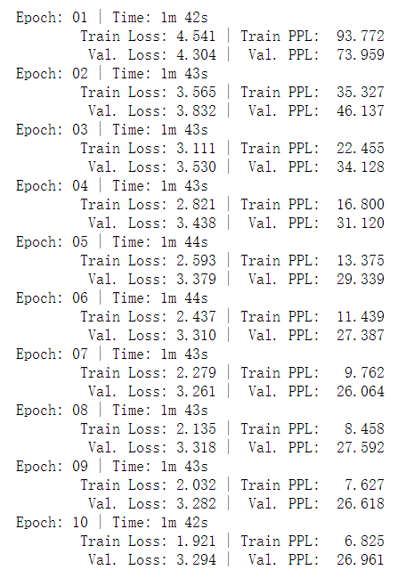
    return lossAll/len(data_iter)

for epoch in range(epochs):
    start_time = time.time()
    train_loss = train(model,train_iter, optim, criterion,clip=1)
    valid_loss = evaluate(model,val_iter,criterion)
    end_time = time.time()
    epoch_mins, epoch_secs = epoch_time(start_time, end_time)
        
    print(f'Epoch: {epoch+1:02} | Time: {epoch_mins}m {epoch_secs}s')
    print(f'\tTrain Loss: {train_loss:.3f} | Train PPL: {math.exp(train_loss):7.3f}')
    print(f'\t Val. Loss: {valid_loss:.3f} |  Val. PPL: {math.exp(valid_loss):7.3f}')

Experimental results: