Next, I will use three examples to learn the trajectory planning of seventh degree polynomial with you. The first one has a problem and we look forward to solving it together. Is it just caused by the solution of inverse solution? The first model is the GLUON-6L3 manipulator in the previous paper
clear;clc;close all;
% DH Modeling part theta,   d,       a,   alpha
L(1)=Link([  0,    0.1015,     0,        0],'modified');
L(2)=Link([  0,    0.0792,     0,    -pi/2],'modified');
L(3)=Link([  0,    -0.0792,   0.173,     0],'modified');
L(4)=Link([  0,    0.0792,    0.173,     0],'modified');
L(5)=Link([  0,    0.0792,     0,     pi/2],'modified');
L(6)=Link([  0,    0.0417,     0,    -pi/2],'modified');

L(2).offset=-pi/2; %Set joint variable offset
L(4).offset=pi/2;

robot= SerialLink(L, 'name', 'GLUON_6L3');  %Establish the manipulator model

%Adjust coordinate axis and field of view
set(gca,'XLim',[-0.6,0.6]);  %take X The axis range is set to[-400,400]
set(gca,'YLim',[-0.6,0.6]);  %take X The axis range is set to[-500,500]
set(gca,'ZLim',[0,0.6]);      %take Z The axis range is set to[0,600],The minimum value is set to 0 to eliminate the long rod under the model
set(gca,'XDir','reverse');    %take x The axis direction is set to reverse
set(gca,'YDir','reverse');    %take Y The axis direction is set to reverse
set(gca,'View',[-85,10]);     %Set the field of view direction angle and pitch angle

%Set joint variable range
L(1).qlim=[deg2rad(-140) deg2rad(140)];
L(2).qlim=[deg2rad(-90)   deg2rad(90)];
L(3).qlim=[deg2rad(-140) deg2rad(140)];
L(4).qlim=[deg2rad(-140) deg2rad(140)];
L(5).qlim=[deg2rad(-140) deg2rad(140)];
L(6).qlim=[deg2rad(-360) deg2rad(360)];

t0 = 0;       %Start time
t1 = 2;       %After the second point
t2 = t1 + 4;  %After the third point
tm = t2 + 4;  %Reach the target point

t0_1 = 0:0.5:2;  %First period of time
t1_2 = 0:0.5:4;  %Second period of time
t2_x = 0:0.5:4;  %The third period

%By changing the position of the four points, the trajectory will be re planned
aim0 = [0 0.121 0.527];     %starting point
aim1 = [0.25 0.121 0.445];  %First pass point
aim2 = [0.373 0.121 0.306]; %Second pass point
aimx = [0.425 0.121 0.102]; %End

T0 = transl(aim0);   %Convert to homogeneous matrix
T1 = transl(aim1);
T2 = transl(aim2);
Tx = transl(aimx);

%Solve joint angles at four locations,It's used here ikine()Inverse solution
theta0 = robot.ikine(T0);
theta1 = robot.ikine(T1);
theta2 = robot.ikine(T2);
thetax = robot.ikine(Tx);

%initial condition
theta0_ = [0 0 0 0 0 0];   %Speed at initial position
theta0__ = [0 0 0 0 0 0];  %Acceleration at initial position
thetax_ = [0 0 0 0 0 0];   %Speed at target position
thetax__ = [0 0 0 0 0 0];  %Acceleration at target position
% Seventh degree polynomial
Theta = [theta0' theta0_' theta0__' theta1' theta2' thetax' thetax_' thetax__']'; % Initial position, position, velocity, acceleration. Target position, velocity, acceleration
M = [1     0    0      0       0        0        0        0
     0     1    0      0       0        0        0        0
     0     0    2      0       0        0        0        0
     1     t1   t1^2   t1^3    t1^4     t1^5     t1^6     t1^7
     1     t2   t2^2   t2^3    t2^4     t2^5     t2^6     t2^7
     1     tm   tm^2   tm^3    tm^4     tm^5     tm^6     tm^7
     0     1    2*tm   3*tm^2  4*tm^3   5*tm^4   6*tm^5   7*tm^6
     0     0    2      6*tm    12*tm^2  20*tm^3  30*tm^4  42*tm^5];

 C = M^-1 * Theta;  %The first i Column corresponds to the second column i Coefficients of the seventh degree polynomial of joints
 k=1;

 %Calculate joint functions
 tmietick= 0.1;     %Simulation step
 T = 0:tmietick:10;

%The following three sentences are used for trajectory planning of seventh degree polynomial
 Q = [ones(int16(10/tmietick)+1,1)   T'    (T.^2)'   (T.^3)'   (T.^4)'   (T.^5)'   (T.^6)'  (T.^7)']*C;  %angle
 Qv =[zeros(int16(10/tmietick)+1,1)  ones(int16(10/tmietick)+1,1) 2* T' 3*(T.^2)' 4*(T.^3)' 5*(T.^4)' 6*(T.^5)' 7*(T.^6)']*C; %speed
 Qa =[zeros(int16(10/tmietick)+1,1)  zeros(int16(10/tmietick)+1,1) 2*ones(int16(10/tmietick)+1,1) 6*T' 12*(T.^2)' 20*(T.^3)' 30*(T.^4)' 42*(T.^5)']*C;%acceleration

 Txy=robot.fkine(Q); %Forward kinematics
 henji=transl(Txy);
 x = henji(:,1);y = henji(:,2);z = henji(:,3);
 figure(1)
 plot3(x,y,z,'r');  %Track image display
 hold on;

[x0,y0,z0]  = ellipsoid(aim0(1),aim0(2),aim0(3),0.05,0.05,0.05);
[x1,y1,z1]  = ellipsoid(aim1(1),aim1(2),aim1(3),0.05,0.05,0.05);
[x2,y2,z2]  = ellipsoid(aim2(1),aim2(2),aim2(3),0.05,0.05,0.05);
[xx,yx,zx]  = ellipsoid(aimx(1),aimx(2),aimx(3),0.05,0.05,0.05);   %Draw four process points
surf(x0,y0,z0) %Draw starting point
surf(x1,y1,z1) %Draw the first passing point
surf(x2,y2,z2) %Draw the second passing point
surf(xx,yx,zx) %Draw target point
hold on;

robot.plot(Q); %Dynamically draw the trajectory

%Draw the curve of joint position, velocity and acceleration
figure(2)
subplot(3,1,1);
plot(T,Q);
title('Joint displacement');xlabel('time t/s');ylabel('displacement s/rad');
legend('Joint 1','Joint 2','Joint 3','Joint 4','Joint 5','Joint 6','location','northeastoutside' );
grid on;

subplot(3,1,2);
plot(T,Qv);
title('Joint velocity');xlabel('time t/s');ylabel('speed v/(rad/s)');
legend('Joint 1','Joint 2','Joint 3','Joint 4','Joint 5','Joint 6','location','northeastoutside' );
grid on;

subplot(3,1,3);
plot(T,Qa);
title('Joint acceleration');xlabel('time t/s');ylabel('acceleration a/(rad/s^2)');
legend('Joint 1','Joint 2','Joint 3','Joint 4','Joint 5','Joint 6','location','northeastoutside' );
grid on;
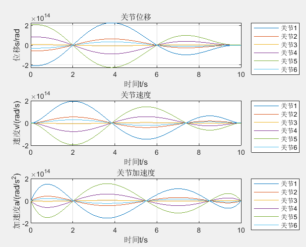
The operation results are as follows:
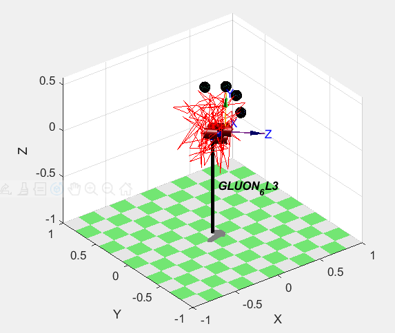
You can see that the trajectory is very disordered
Note: all simulation environments matlab2020B, robot toolbox 9.10
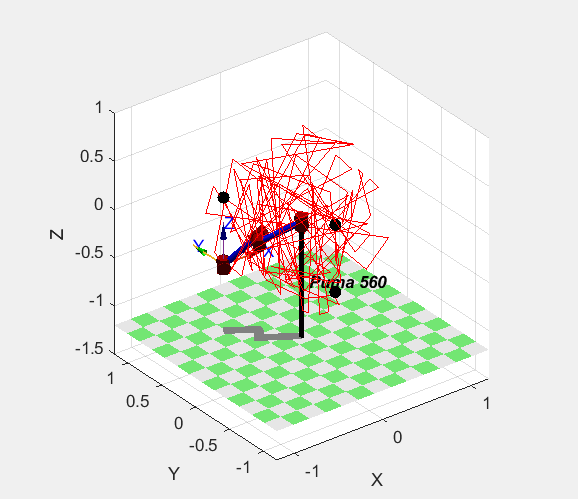
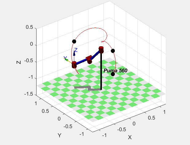
If the model is replaced with PUMA560 robot.
clear;clc;close all;

mdl_puma560;  %Load in the robot toolbox puma560 Model. Later, the reference model only needs to be p560.Form of
t0 = 0;       %Start time
t1 = 2;       %After the second point
t2 = t1 + 4;  %After the third point
tm = t2 + 4;  %Reach the target point

t0_1 = 0:0.2:2;  %First period of time
t1_2 = 0:0.5:4;  %Second period of time
t2_x = 0:0.3:4;  %The third period

aim0 = [0,-0.5,-0.5];   %starting point
aim1 = [0,-0.5,0.2];    %First pass point
aim2 = [-0.5,0.5,0.2];  %Second pass point
aimx = [-0.5,0.5,-0.5]; %End

T0 = transl(aim0);   %Convert to homogeneous matrix
T1 = transl(aim1);
T2 = transl(aim2);
Tx = transl(aimx);

%Solve joint angles at four locations
theta0 = p560.ikine(T0);
theta1 = p560.ikine(T1);
theta2 = p560.ikine(T2);
thetax = p560.ikine(Tx);

%initial condition
theta0_ = [0 0 0 0 0 0];   %Speed at initial position
theta0__ = [0 0 0 0 0 0];  %Acceleration at initial position
thetax_ = [0 0 0 0 0 0];   %Speed at target position
thetax__ = [0 0 0 0 0 0];  %Acceleration at target position
Theta = [theta0' theta0_' theta0__' theta1' theta2' thetax' thetax_' thetax__']';%Initial position, position, velocity, acceleration. Target position, velocity, acceleration
M = [1     0    0      0       0        0        0        0
     0     1    0      0       0        0        0        0
     0     0    2      0       0        0        0        0
     1     t1   t1^2   t1^3    t1^4     t1^5     t1^6     t1^7
     1     t2   t2^2   t2^3    t2^4     t2^5     t2^6     t2^7
     1     tm   tm^2   tm^3    tm^4     tm^5     tm^6     tm^7
     0     1    2*tm   3*tm^2  4*tm^3   5*tm^4   6*tm^5   7*tm^6
     0     0    2      6*tm    12*tm^2  20*tm^3  30*tm^4  42*tm^5];
 C = M^-1 * Theta;  %The first i Column corresponds to the second column i Coefficients of the seventh degree polynomial of joints
 k=1;
 %Calculate joint functions
 tmietick = 0.1;  %Simulation step
 T = 0: tmietick:10;
 Q = [ones(int16(10/tmietick)+1,1)   T'    (T.^2)'   (T.^3)'   (T.^4)'   (T.^5)'   (T.^6)'  (T.^7)']*C;  %angle
 Qv =[zeros(int16(10/tmietick)+1,1)  ones(int16(10/tmietick)+1,1) 2* T' 3*(T.^2)' 4*(T.^3)' 5*(T.^4)' 6*(T.^5)' 7*(T.^6)']*C; %speed
 Qa =[zeros(int16(10/tmietick)+1,1)  zeros(int16(10/tmietick)+1,1) 2*ones(int16(10/tmietick)+1,1) 6*T' 12*(T.^2)' 20*(T.^3)' 30*(T.^4)' 42*(T.^5)']*C;%acceleration

 Txy=p560.fkine(Q); %Forward kinematics analysis
 henji=transl(Txy);
 x = henji(:,1);y = henji(:,2);z = henji(:,3);
 figure(1)
%  waitforbuttonpress;
 plot3(x,y,z,'r');  %Track image display
 hold on;

[x0,y0,z0]  = ellipsoid(aim0(1),aim0(2),aim0(3),0.05,0.05,0.05);
[x1,y1,z1]  = ellipsoid(aim1(1),aim1(2),aim1(3),0.05,0.05,0.05);
[x2,y2,z2]  = ellipsoid(aim2(1),aim2(2),aim2(3),0.05,0.05,0.05);
[xx,yx,zx]  = ellipsoid(aimx(1),aimx(2),aimx(3),0.05,0.05,0.05); %Draw four process points
surf(x0,y0,z0) %Draw starting point
surf(x1,y1,z1) %Draw the first passing point
surf(x2,y2,z2) %Draw the second passing point
surf(xx,yx,zx) %Draw target point
hold on;

p560.plot(Q); %Dynamically draw the trajectory

%Draw the curve of joint position, velocity and acceleration
figure(2)
subplot(3,1,1);
plot(T,Q);
title('Joint displacement');xlabel('time t/s');ylabel('displacement s/rad');
legend('Joint 1','Joint 2','Joint 3','Joint 4','Joint 5','Joint 6','location','northeastoutside' );
grid on;

subplot(3,1,2);
plot(T,Qv);
title('Joint velocity');xlabel('time t/s');ylabel('speed v/(rad/s)');
legend('Joint 1','Joint 2','Joint 3','Joint 4','Joint 5','Joint 6','location','northeastoutside' );
grid on;

subplot(3,1,3);
plot(T,Qa);
title('Joint acceleration');xlabel('time t/s');ylabel('acceleration a/(rad/s^2)');
legend('Joint 1','Joint 2','Joint 3','Joint 4','Joint 5','Joint 6','location','northeastoutside' );
grid on;
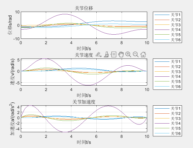
The result is as follows. It is still disordered
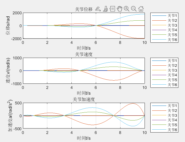
However, just make a little modification to the inverse solution.
%The program implements the robot toolbox puma560 The model is used for quadratic polynomial four-point trajectory planning. The trajectory is displayed separately from the angular position, velocity and acceleration of each joint, and is not drawn in real time
clear;clc;close all;

mdl_puma560;  %Load in the robot toolbox puma560 Model. Later, the reference model only needs to be p560.Form of
t0 = 0;       %Start time
t1 = 2;       %After the second point
t2 = t1 + 4;  %After the third point
tm = t2 + 4;  %Reach the target point

t0_1 = 0:0.2:2;  %First period of time
t1_2 = 0:0.5:4;  %Second period of time
t2_x = 0:0.3:4;  %The third period

aim0 = [0,-0.5,-0.5];   %starting point
aim1 = [0,-0.5,0.2];    %First pass point
aim2 = [-0.5,0.5,0.2];  %Second pass point
aimx = [-0.5,0.5,-0.5]; %End

T0 = transl(aim0);   %Convert to homogeneous matrix
T1 = transl(aim1);
T2 = transl(aim2);
Tx = transl(aimx);

%Solve joint angles at four locations
theta0 = p560.ikine6s(T0,'rdf'); %Left arm, elbow down, wrist turned(Rotate 180 degrees)
theta1 = p560.ikine6s(T1,'rdf');
theta2 = p560.ikine6s(T2,'rdf');
thetax = p560.ikine6s(Tx,'rdf');

%initial condition
theta0_ = [0 0 0 0 0 0];   %Speed at initial position
theta0__ = [0 0 0 0 0 0];  %Acceleration at initial position
thetax_ = [0 0 0 0 0 0];   %Speed at target position
thetax__ = [0 0 0 0 0 0];  %Acceleration at target position
Theta = [theta0' theta0_' theta0__' theta1' theta2' thetax' thetax_' thetax__']';%Initial position, position, velocity, acceleration. Target position, velocity, acceleration
M = [1     0    0      0       0        0        0        0
     0     1    0      0       0        0        0        0
     0     0    2      0       0        0        0        0
     1     t1   t1^2   t1^3    t1^4     t1^5     t1^6     t1^7
     1     t2   t2^2   t2^3    t2^4     t2^5     t2^6     t2^7
     1     tm   tm^2   tm^3    tm^4     tm^5     tm^6     tm^7
     0     1    2*tm   3*tm^2  4*tm^3   5*tm^4   6*tm^5   7*tm^6
     0     0    2      6*tm    12*tm^2  20*tm^3  30*tm^4  42*tm^5];
 C = M^-1 * Theta;  %The first i Column corresponds to the second column i Coefficients of the seventh degree polynomial of joints
 k=1;
 %Calculate joint functions
 tmietick = 0.1;  %Simulation step
 T = 0: tmietick:10;
 Q = [ones(int16(10/tmietick)+1,1)   T'    (T.^2)'   (T.^3)'   (T.^4)'   (T.^5)'   (T.^6)'  (T.^7)']*C;  %angle
 Qv =[zeros(int16(10/tmietick)+1,1)  ones(int16(10/tmietick)+1,1) 2* T' 3*(T.^2)' 4*(T.^3)' 5*(T.^4)' 6*(T.^5)' 7*(T.^6)']*C; %speed
 Qa =[zeros(int16(10/tmietick)+1,1)  zeros(int16(10/tmietick)+1,1) 2*ones(int16(10/tmietick)+1,1) 6*T' 12*(T.^2)' 20*(T.^3)' 30*(T.^4)' 42*(T.^5)']*C;%acceleration

 Txy=p560.fkine(Q); %Forward kinematics analysis
 henji=transl(Txy);
 x = henji(:,1);y = henji(:,2);z = henji(:,3);
 figure(1)
%  waitforbuttonpress;
 plot3(x,y,z,'r');  %Track image display
 hold on;

[x0,y0,z0]  = ellipsoid(aim0(1),aim0(2),aim0(3),0.05,0.05,0.05);
[x1,y1,z1]  = ellipsoid(aim1(1),aim1(2),aim1(3),0.05,0.05,0.05);
[x2,y2,z2]  = ellipsoid(aim2(1),aim2(2),aim2(3),0.05,0.05,0.05);
[xx,yx,zx]  = ellipsoid(aimx(1),aimx(2),aimx(3),0.05,0.05,0.05); %Draw four process points
surf(x0,y0,z0) %Draw starting point
surf(x1,y1,z1) %Draw the first passing point
surf(x2,y2,z2) %Draw the second passing point
surf(xx,yx,zx) %Draw target point
hold on;

p560.plot(Q); %Dynamically draw the trajectory

%Draw the curve of joint position, velocity and acceleration
figure(2)
subplot(3,1,1);
plot(T,Q);
title('Joint displacement');xlabel('time t/s');ylabel('displacement s/rad');
legend('Joint 1','Joint 2','Joint 3','Joint 4','Joint 5','Joint 6','location','northeastoutside' );
grid on;

subplot(3,1,2);
plot(T,Qv);
title('Joint velocity');xlabel('time t/s');ylabel('speed v/(rad/s)');
legend('Joint 1','Joint 2','Joint 3','Joint 4','Joint 5','Joint 6','location','northeastoutside' );
grid on;

subplot(3,1,3);
plot(T,Qa);
title('Joint acceleration');xlabel('time t/s');ylabel('acceleration a/(rad/s^2)');
legend('Joint 1','Joint 2','Joint 3','Joint 4','Joint 5','Joint 6','location','northeastoutside' );
grid on;
The results are shown in the figure below
Just modify the following sentences, the trajectory will be beautiful: then I have a question, where is the function of ikine() in the robot toolbox? Is that why I have to push the inverse solution and write the inverse solution function myself?
theta0 = p560.ikine6s(T0,'rdf'); %Left arm, elbow down, wrist turned(Rotate 180 degrees)
theta1 = p560.ikine6s(T1,'rdf');
theta2 = p560.ikine6s(T2,'rdf');
thetax = p560.ikine6s(Tx,'rdf');
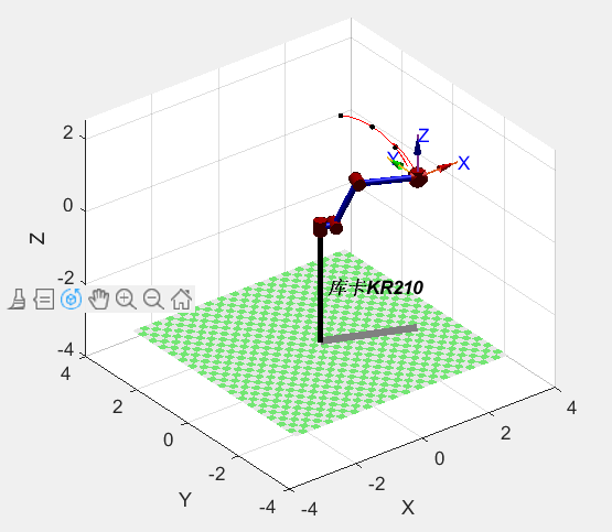
Next, I tried to save the KUKA robot
clear;clc;close all;
%DH Parameters: d Connecting rod offset;   a: Rod length;     alpha: Connecting rod angle;  offset;Show the appearance of the Department'standard' or 'modified'
L1=Link('d',0,        'a',0,         'alpha',0,                           'modified');  %use Link Function to create a single joint
L2=Link('d',0,        'a',0.350,     'alpha',-pi/2,     'offset',-pi/2,   'modified');  %Command window input help Link View function usage
L3=Link('d',0,        'a',1.250,     'alpha',0,                           'modified');
L4=Link('d',1.500,     'a',-0.055,   'alpha',-pi/2,     'offset',0,      'modified');
L5=Link('d',0,        'a',0,         'alpha',pi/2,                        'modified');
L6=Link('d',0,        'a',0,         'alpha',-pi/2,                       'modified');
robot=SerialLink([L1 L2 L3 L4 L5 L6],'name','KUKA KR210') ;  %use SerialLink Function to establish the robot model and input in the command window help Link View function usage
%********The following three sentences are for using the positive solution function in the robot toolbox**********%
Theta=[45 45 45 45 60 30];
Theta=Theta/180*pi;    %When above theta When the input is radian system, this sentence does not need to be used
% T16=robot.fkine(Theta); %Robot toolbox fkine Homogeneous transformation of positive solution of function. Change above theta The internal value and pose value will change
W=[-3,+3,-3,+3,-3,+8];         %Length of three axis six direction coordinate system
figure(1);                                       %Open a new picture window
robot.plot(Theta,'tilesize',0.15,'workspace',W);  %Draw a 3D model to display the current input theta horn

t0 = 0;       %Start time
t1 = 2;       %After the second point
t2 = t1 + 4;  %After the third point
tm = t2 + 4;  %Reach the target point

t0_1 = 0:0.2:2;  %First period of time
t1_2 = 0:0.5:4;  %Second period of time
t2_x = 0:0.3:4;  %The third period

%By changing the position of the four points, the trajectory will be re planned 4
aim0 = [1.0,0.5,2.5];    %starting point
aim1 = [1.8,0.3,2.0];    %First pass point
aim2 = [2.17,-0.12,1.5]; %Second pass point
aimx = [2.24,-0.9,1];    %End

T0 = transl(aim0);   %Convert to homogeneous matrix
T1 = transl(aim1);
T2 = transl(aim2);
Tx = transl(aimx);

%Solve joint angles at four locations,You can't use them all here ikine()Inverse solution
theta0 = robot.ikine(T0);
theta1 = robot.ikcon(T1,theta0);
theta2 = robot.ikcon(T2,theta1);
thetax = robot.ikcon(Tx,theta2);

%initial condition
theta0_ = [0 0 0 0 0 0];   %Speed at initial position
theta0__ = [0 0 0 0 0 0];  %Acceleration at initial position
thetax_ = [0 0 0 0 0 0];   %Speed at target position
thetax__ = [0 0 0 0 0 0];  %Acceleration at target position
Theta = [theta0' theta0_' theta0__' theta1' theta2' thetax' thetax_' thetax__']';%Initial position, position, velocity, acceleration. Target position, velocity, acceleration
M = [1     0    0      0       0        0        0        0
     0     1    0      0       0        0        0        0
     0     0    2      0       0        0        0        0
     1     t1   t1^2   t1^3    t1^4     t1^5     t1^6     t1^7
     1     t2   t2^2   t2^3    t2^4     t2^5     t2^6     t2^7
     1     tm   tm^2   tm^3    tm^4     tm^5     tm^6     tm^7
     0     1    2*tm   3*tm^2  4*tm^3   5*tm^4   6*tm^5   7*tm^6
     0     0    2      6*tm    12*tm^2  20*tm^3  30*tm^4  42*tm^5];
 C = M^-1 * Theta;  %The first i Column corresponds to the second column i Coefficients of the seventh degree polynomial of joints
 k=1;

 %Calculate joint functions
 tmietick= 0.1;  %Simulation step
 T = 0:tmietick:10;
 Q = [ones(int16(10/tmietick)+1,1)   T'    (T.^2)'   (T.^3)'   (T.^4)'   (T.^5)'   (T.^6)'  (T.^7)']*C;  %angle
 Qv =[zeros(int16(10/tmietick)+1,1)  ones(int16(10/tmietick)+1,1) 2* T' 3*(T.^2)' 4*(T.^3)' 5*(T.^4)' 6*(T.^5)' 7*(T.^6)']*C; %speed
 Qa =[zeros(int16(10/tmietick)+1,1)  zeros(int16(10/tmietick)+1,1) 2*ones(int16(10/tmietick)+1,1) 6*T' 12*(T.^2)' 20*(T.^3)' 30*(T.^4)' 42*(T.^5)']*C;%acceleration

 Txy=robot.fkine(Q); %Forward kinematics analysis
 henji=transl(Txy);
 x = henji(:,1);y = henji(:,2);z = henji(:,3);
 figure(1)
%  waitforbuttonpress;
 plot3(x,y,z,'r');  %Track image display
 hold on;

[x0,y0,z0]  = ellipsoid(aim0(1),aim0(2),aim0(3),0.05,0.05,0.05);
[x1,y1,z1]  = ellipsoid(aim1(1),aim1(2),aim1(3),0.05,0.05,0.05);
[x2,y2,z2]  = ellipsoid(aim2(1),aim2(2),aim2(3),0.05,0.05,0.05);
[xx,yx,zx]  = ellipsoid(aimx(1),aimx(2),aimx(3),0.05,0.05,0.05); %Draw four process points
surf(x0,y0,z0) %Draw starting point
surf(x1,y1,z1) %Draw the first passing point
surf(x2,y2,z2) %Draw the second passing point
surf(xx,yx,zx) %Draw target point
hold on;

robot.plot(Q); %Dynamically draw the trajectory

%Draw the curve of joint position, velocity and acceleration
figure(2)
subplot(3,1,1);
plot(T,Q);
title('Joint displacement');xlabel('time t/s');ylabel('displacement s/rad');
legend('Joint 1','Joint 2','Joint 3','Joint 4','Joint 5','Joint 6','location','northeastoutside' );
grid on;

subplot(3,1,2);
plot(T,Qv);
title('Joint velocity');xlabel('time t/s');ylabel('speed v/(rad/s)');
legend('Joint 1','Joint 2','Joint 3','Joint 4','Joint 5','Joint 6','location','northeastoutside' );
grid on;

subplot(3,1,3);
plot(T,Qa);
title('Joint acceleration');xlabel('time t/s');ylabel('acceleration a/(rad/s^2)');
legend('Joint 1','Joint 2','Joint 3','Joint 4','Joint 5','Joint 6','location','northeastoutside' );
grid on;
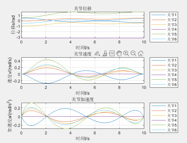
After many twists and turns, a more satisfactory track can be obtained through such modification:
theta0 = robot.ikine(T0);
theta1 = robot.ikcon(T1,theta0);
theta2 = robot.ikcon(T2,theta1);
thetax = robot.ikcon(Tx,theta2);
The operation results are as follows:
But how to combine the first one, ikine(),ikcon(),ikine6s(), is not acceptable. The influence of the inverse solution is still great. I haven't figured out the reason. I hope to discuss it with you. If you know, you can give a solution in the comments or write a blog post to explain it in detail, and look forward to your solution.
Finally, I tried to write my own numerical method to solve the inverse solution to replace the inverse solution function of the toolbox. Although the trajectory is perfect, I still feel that there is something wrong. It should be the optimization of the inverse solution. What rules should be used to select the most suitable solution from the eight groups of solutions needs to be studied.
Note: the planning code of the second example comes from a CSDN blogger. Thank you for your work, but I forgot his blog name and found it later.