regression analysis
According to the number of dependent variables and the type of regression function (linear or non-linear), regression methods can be divided into one-variable linear regression, one-variable non-linear regression and multiple regression.
Simple rough understanding: It can be understood as the process of finding an optimal linear mapping function from feature space X to output space Y.
(There's no need to struggle with defining a person, just know that it's something that will work.)
Highlights: Regarding linear and non-linear regression, I summarized a lot of knowledge points in the code. There will be many explanations at the beginning of each piece of code, parameter explanations and knowledge points. It is suggested that we look at more explanations at the beginning of the code.
Univariate linear regression
For linear regression of one variable, a simple rough understanding is to give a bunch of points, (x1,y1), (x2,y2),... (xn,yn), and then according to the linear regression equation of one variable (fixed) to solve the process of beta 0, beta 1, the linear regression equation of one variable is basically the same as that of high school, but before it had to be calculated by human, now it can be calculated by matlab.
Understanding the case (MATLAB Mathematical Modeling Method and Practice (3rd Edition) page 48):
This is a classical one-dimensional regression problem. According to the given point, the process of calculating regression coefficients is given. Here we give the code, focusing on the knowledge points and parameter descriptions in the code, at the beginning of each formal code.
% % % % % % % % % % % % % % % % % % % % % % % % % % % % % % % % % % % % % % % % % % % % % % % % % % % % % % % % % % % % % % % % % % %
% Regression analysis is a mathematical method to deal with the correlation between variables. The general methods and steps to solve the problem are as follows:
%               (1)Collect a set of data including dependent and independent variables.
%               (2)Select the model between dependent variable and independent variable, that is, a mathematical formula, using data to calculate the coefficients of the model according to the least square criterion.
%               (3)The statistical analysis method is used to compare the different models and find out the best fitting model with the data.
%               (4)Determine whether the model is suitable for this set of data;
%               (5)The model is used to predict or explain dependent variables.
%
% Univariate linear regression equation:
%                   y = β0 + β1*x;  βFor regression coefficient
%
%
% matlab Module description:
% (1)plot(x,y,'r*');
% (2)n = length(x),X=[ones(n,1),x'];
% (3)Y = y';
% (4)[b,bint,r,rint,s]=regress(Y,X,alpha);
% Description of parameters: plot(x,y,'r*'):Drawing scatter plots
%           X:From the given x Value determination, ( X Must be a column matrix, so if x A row matrix must be passed x'Converted to column vectors)
%           Y:From the given y Value determination, ( Y Must be a column matrix, so if y A row matrix must be passed y'Converted to column vectors)
%           alpha:Significance level(Default 0 by default.05)
%           b:Set of correlation coefficients, linear regression of one variable, b There are two values. b(1,1) = β0,b(2,1) = β1
%           bint: Interval Estimation of Regression Coefficient
%           r :residual
%           rint :Residual confidence interval
%           s :The statistics used to test regression models have four values: correlation coefficient. R^2,F Value, and F Corresponding probability p,Error variance.
%           Be careful: s Usually used for model checking,1.Relational Number R^2 The closer to 1, the more significant the regression equation is.
%                                       2.p<alpha When, refuse H0,Establishment of regression model
%                                       3.F > F1-alpha(k,n-k-1)[Through this function finv(1-,1, n-2)Reject when you get _____________ H0,F The larger the regression equation is, the more significant the regression equation is.,among F1-alpha(k,n-k-1)The values are available F Distribution tables, or direct use MATLAB command finv(1-,1, n-2)Calculated
% (4)Residual analysis: rcoplot(r,rint)
%             The plotted graph, whose red dots are abnormal data, can be removed and then re-calculated for linear regression analysis of one variable.
%
%
% matlab Realization:
% (1)Input:
%         x(1*n)Matrix Storage x coordinate
%         y(1*n)Matrix Storage y coordinate
% (2)Output:
%         [b,bint,r,rint,s]=regress(Y,X,alpha);All the parameters, regression coefficients b Constituting a Univariate Regression Model
%         Residual Graph Analysis
%
% Focus: If something goes wrong;"Misuse horzcat Dimensional inconsistency of series matrices"It may be X,Y There are problems with the transformation of row matrix and column matrix.
% % % % % % % % % % % % % % % % % % % % % % % % % % % % % % % % % % % % % % % % % % % % % % % % % % % % % % % % % % % % % % % % % %


clc
% Data storage
% x = [3.5 5.3 5.1 5.8 4.2 6.0 6.8 5.5 3.1 7.2 4.5 4.9 8.0 6.5 6.6 3.7 6.2 7.0 4.0 4.5 5.9 5.6 4.8 3.9];
% y = [33.2 40.3 38.7 46.8 41.4 37.5 39.0 40.7 30.1 52.9 38.2 31.8 43.3 44.1 42.5 33.6 34.2 48.0 38.0 35.9 40.4 36.8 45.2 35.1];

x=[23.80,27.60,31.60,32.40,33.70,34.90,43.20,52.80,63.80,73.40];
y=[41.4,51.8,61.70,67.90,68.70,77.50,95.90,137.40,155.0,175.0];

% Drawing scatter plots
% plot(x,y,'r*');

% Length of data
n=length(x);

% X,Y Make
X=[ones(n,1),x'];
Y = y';

 % linear analysis
[b,bint,r,rint,s]=regress(Y,X,0.05);
b
bint
% r
% rint
s

% Residual analysis
figure;
rcoplot(r,rint);


fprintf('The fitting function is: f(x) = %d + %d*x\n',b(1,1),b(2,1));
figure
f = @(x) b(1,1) + b(2,1) * x;
plot(x,y,'r*');
hold on;
ezplot(f, [0, 90]);             % Draw a function image
title('Fitted curve');
Operation results: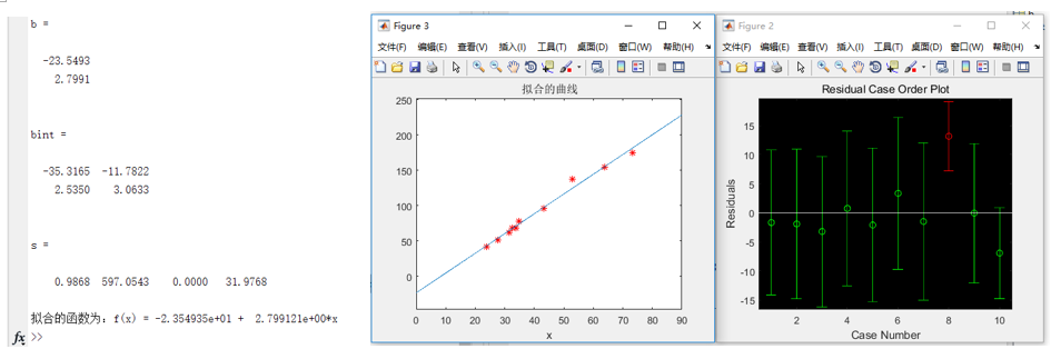
As for the parameters in the running result, b, bint, r, rint, s and so on are explained at the beginning of the above code. This is very important. It is suggested that we take a look at it more.
multiple linear regression
In regression analysis, if there are two or more independent variables, it is called multiple regression. For multivariate linear regression, compared with univariate linear regression, the regression coefficients are only more, the independent variables are more, and the others are almost the same. In the same way, give a bunch of points, but these points correspond to more independent variables (more than two), the process of solving partial regression coefficient.
Case (MATLAB Mathematical Modeling Method and Practice (3rd Edition) page 52):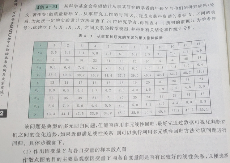
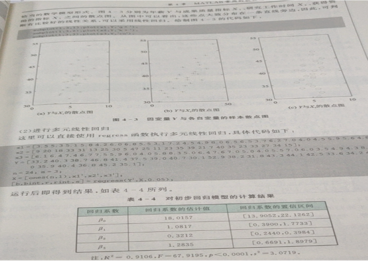
The second picture above is the idea of solving problems in the book (if you are bored, you can not read it). Here is the code.
% % % % % % % % % % % % % % % % % % % % % % % % % % % % % % % % % % % % % % % % % % % % % % % % % % % % % % % % % % % % % % % % % % %
% Regression analysis is a mathematical method to deal with the correlation between variables. The general methods and steps to solve the problem are as follows:
%               (1)Collect a set of data including dependent and independent variables.
%               (2)By drawing scatter plots, we can judge whether the regression is in line with the linear regression and decide which kind of linear regression to use.
%               (3)Select the model between dependent variable and independent variable, that is, a mathematical formula, using data to calculate the coefficients of the model according to the least square criterion.
%               (4)The statistical analysis method is used to compare the different models and find out the best fitting model with the data.
%               (5)Determine whether the model is suitable for this set of data;
%               (5)The model is used to predict or explain dependent variables.
%
% Multivariate linear regression equation: y=b0+b1X1+b2X2+...+bnXn
%                   b0 Constant term
%                   b1,b2,b3,...bn Be called y Corresponding to x1,x2,x3,...xn Partial regression coefficient
%
%
% matlab Module description:
% (1)subplot(1,3,1),plot(x1,y,'g*'),
%    subplot(1,3,2),plot(x2,y,'k+'),
%    subplot(1,3,3),plot(x3,y,'ro'),
%    ......
% (2)n = length(x1),X=[ones(n,1),x1',x2',x3',...];
% (3)Y = y';
% (4)[b,bint,r,rint,s]=regress(Y,X,alpha);
% Description of parameters: subplot(1,3,1),plot(x1,y,'g*'):Drawing scatter plots
%           X:From the given x Value determination, ( X Must be a column matrix, so if x A row matrix must be passed x'Converted to column vectors)
%           Y:From the given y Value determination, ( Y Must be a column matrix, so if y A row matrix must be passed y'Converted to column vectors)
%           alpha:Significance level(Default 0 by default.05)
%           b:Set of correlation coefficients, linear regression of one variable, b There are two values. b(1,1) = β0,b(2,1) = β1
%           bint: Interval Estimation of Regression Coefficient
%           r :residual
%           rint :Residual confidence interval
%           s :The statistics used to test regression models have four values: correlation coefficient. R^2,F Value, and F Corresponding probability p,Error variance.
%           Be careful: s Usually used for model checking,1.Relational Number R^2 The closer to 1, the more significant the regression equation is.
%                                       2.p<alpha When, refuse H0,Establishment of regression model
%                                       3.F > F1-alpha(k,n-k-1)[Through this function finv(1-,1, n-2)Reject when you get _____________ H0,F The larger the regression equation is, the more significant the regression equation is.,among F1-alpha(k,n-k-1)The values are available F Distribution tables, or direct use MATLAB command finv(1-,1, n-2)Calculated
% (4)Residual analysis: rcoplot(r,rint)
%             The plotted graph, whose red dots are abnormal data, can be removed and then re-calculated for linear regression analysis of one variable.
%
%
% matlab Realization:
% (1)Input:
%         x1(1*n)Matrix Storage x1 coordinate
%         x2(1*n)Matrix Storage x2 coordinate
%         ......
%         y1(1*n)Matrix Storage y coordinate
%         y2(1*n)Matrix Storage y2 coordinate
%         ......
% (2)Output:
%         [b,bint,r,rint,s]=regress(Y,X,alpha);All the parameters, regression coefficients b Constituting a multivariate regression model
%         Residual Graph Analysis
%
% Focus: If something goes wrong;"Misuse horzcat Dimensional inconsistency of series matrices"It may be X,Y There are problems with the transformation of row matrix and column matrix.
% % % % % % % % % % % % % % % % % % % % % % % % % % % % % % % % % % % % % % % % % % % % % % % % % % % % % % % % % % % % % % % % % %


clc
% Data storage
x1 = [3.5 5.3 5.1 5.8 4.2 6.0 6.8 5.5 3.1 7.2 4.5 4.9 8.0 6.5 6.6 3.7 6.2 7.0 4.0 4.5 5.9 5.6 4.8 3.9];
x2 = [9 20 18 33 31 13 25 30 5 47 25 11 23 35 39 21 7 40 35 23 33 27 34 15];
x3 = [6.1 6.4 7.4 6.7 7.5 5.9 6.0 4.0 5.8 8.3 5.0 6.4 7.6 7.0 5.0 4.4 5.5 7.0 6.0 3.5 4.9 4.3 8.0 5.8];
y = [33.2 40.3 38.7 46.8 41.4 37.5 39.0 40.7 30.1 52.9 38.2 31.8 43.3 44.1 42.5 33.6 34.2 48.0 38.0 35.9 40.4 36.8 45.2 35.1];

% Drawing scatter plots
subplot(1,3,1);plot(x1,y,'g*');
subplot(1,3,2);plot(x2,y,'k+');
subplot(1,3,3);plot(x3,y,'ro');

% Length of data
n=length(x1);

% X,Y Make
X=[ones(n,1),x1',x2',x3'];
Y = y';

% linear analysis
[b,bint,r,rint,s]=regress(Y,X,0.05);
b
bint
% r
% rint
s

% Residual analysis
rcoplot(r,rint);
Operation results: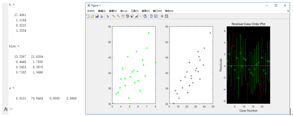
As for the parameters in the running result, b, bint, r, rint, s and so on are explained at the beginning of the above code. This is very important. It is suggested that we take a look at it more.
Univariate Nonlinear Regression
Nonlinear regression is the regression of regression function with non-linear structure about unknown regression coefficients. Simple understanding is that non-linear regression is curve regression.
When making non-linear regression, it is generally necessary to determine the non-linear regression model first and then do non-linear regression; the idea of solving the problem is to draw the given data points through matlab plotting, and then to see which non-linear regression model the scatter plot is more in line with, choose the model, and finally do non-linear regression. Analysis.
Regarding the model, here are some tidies for you:
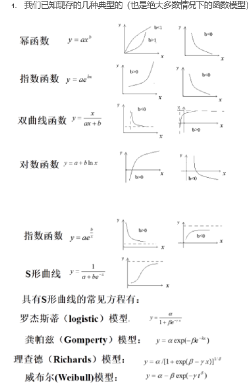
Other non-linear regression models can be searched online by themselves.
Case (MATLAB Mathematical Modeling Method and Practice (3rd Edition) page 50):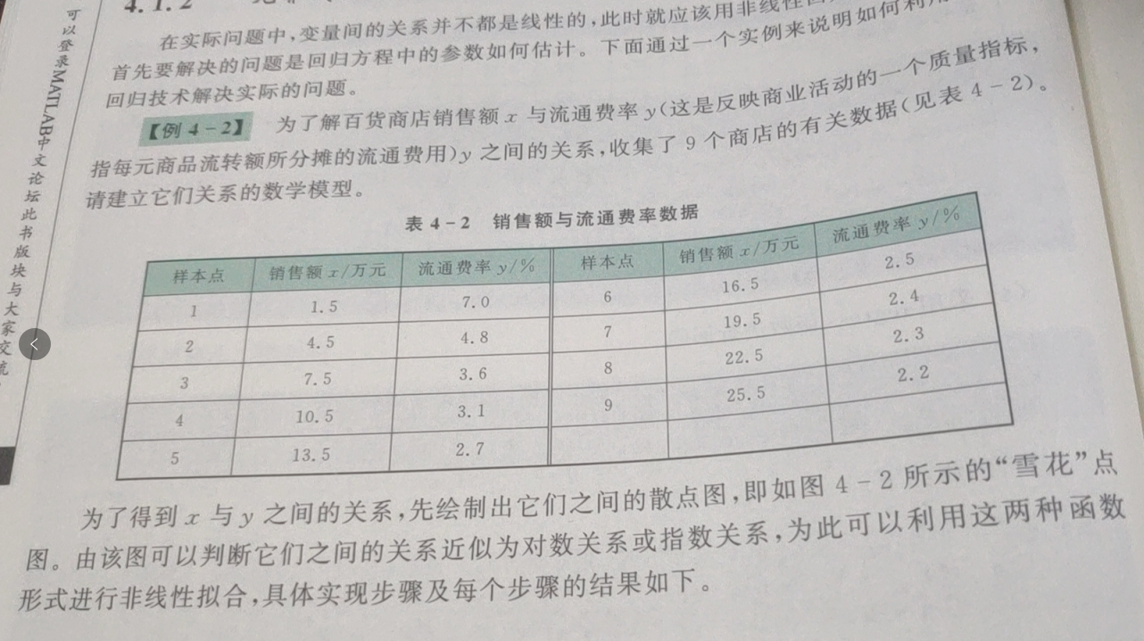
Code:
% % % % % % % % % % % % % % % % % % % % % % % % % % % % % % % % % % % % % % % % % % % % % % % % % % % % % % % % % % % % % % % % % %
% matlab Module introduction:
%   [beta,r]=nlinfit(x,y,'fun1',beta0);
%   beta That is, the required correlation coefficient.
%   r For residual
%   x For data x Axis coordinates, n*m Matrix storage, when x How many hours( x1,x2,x3...),Each group x For a column, x1 For column 1,x2 For the second column, x3 For the third column...Form n*m Matrix of
%   y For data y Axis coordinates,Stored as column matrices
%   fun1 For the expression of a functional model, it is generally necessary to determine the model first and then make a non-linear regression. The function is usually used separately..m File storage,Or define it by yourself
%   beta0 For the initial values of multiple correlation coefficients, the coefficients need to be guessed by themselves, and then the final coefficients can be calculated step by step iteratively from the initial values.
%
% % % % % % % % % % % % % % % % % % % % % % % % % % % % % % % % % % % % % % % % % % % % % % % % % % % % % % % % % % % % % % % % % %
clc
% Data:
x=[1.5, 4.5, 7.5,10.5,13.5,16.5,19.5,22.5,25.5]';
y=[7.0,4.8,3.6,3.1,2.7,2.5,2.4,2.3,2.2]';


%% Logarithmic model fitting: f(x) = b(1) + b(2)*log(x)
myfunc = inline('beta(1)+beta(2)*log(x)','beta','x');%The three parameters are: function model(Note the need to use point division and point multiplication),Undetermined coefficient, independent variable

beta0 = [0.2,0.2]';%Pre-estimation of undetermined coefficients,Fixed and unchangeable

% beta To obtain the correlation coefficient
beta = nlinfit(x,y,myfunc,beta0);

figure;
plot(x,y,'.');
hold on%Guarantee simultaneous display

x = 0:0.01:8;
y = beta(1)+beta(2)*log(x);

plot(x,y);
title('Logarithmic Model Fitting');

%% Exponential model fitting: f(x) = b1*x^b2;
% myfunc = inline('beta(1)*x.^beta(2)','beta','x');%The three parameters are: function model(Note the need to use point division and point multiplication),Undetermined coefficient, independent variable
%
% beta0 = [0.2,0.2]';%Pre-estimation of undetermined coefficients,Fixed and unchangeable
%
% % beta To obtain the correlation coefficient
% beta = nlinfit(x,y,myfunc,beta0);
%
% figure;
% plot(x,y,'.');
% hold on%Guarantee simultaneous display
%
% x = 0:0.01:8;
% y = beta(1)*x.^beta(2);
%
% plot(x,y);
% title('Exponential Model Fitting');
The above two models can only run independently, running one annotated the other.
Operation results: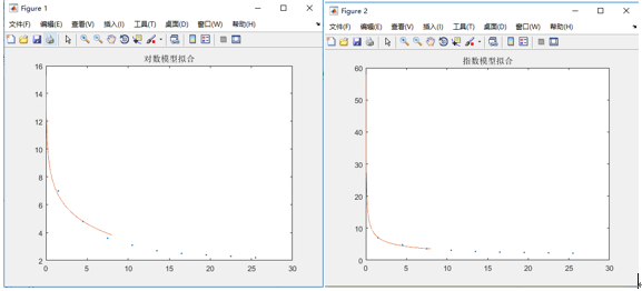
It's important to see where the parameters in the running results are at the beginning of the above code. It's recommended that you take a look at them more.
The above is the whole content. If there are any mistakes, I hope you can criticize and correct them.