Examples

Take the following linear programming as an example 2 x 1 + 3 x 2 − 5 x 3 2x_1 + 3x_2 - 5x_3 2x1 + 3x2 − 5x3 min

m i n z = 2 x 1 + 3 x 2 − 5 x 3 s . t . = { x 1 + x 2 + x 3 = 7 2 x 1 − 5 x 2 + x 3 > = 10 x 1 + 3 x 2 + x 3 < = 12 x 1 , x 2 , x 3 > = 0 min z = 2x_1 + 3x_2 - 5x_3\\ s.t. = \begin{cases} x_1 + x_2 + x_3 = 7 \\ 2x_1 - 5x_2 + x_3 >= 10\\ x_1 + 3x_2 + x_3 <= 12\\ x_1,x_2,x_3 >= 0 \end{cases} minz=2x1​+3x2​−5x3​s.t.=⎩⎪⎪⎪⎨⎪⎪⎪⎧​x1​+x2​+x3​=72x1​−5x2​+x3​>=10x1​+3x2​+x3​<=12x1​,x2​,x3​>=0​

Method 1: use scipy Library

Preparatory knowledge

scipy.optimize.linprog

grammar
scipy.optimize.linprog(c, A_ub=None, b_ub=None, A_eq=None, b_eq=None, bounds=None, method='interior-point', callback=None, options=None, x0=None)

Common parameters:

• c: The coefficient set of the unknowns of the objective function

• A_ub: coefficient set of unknowns on the left of inequality

• B_up, set of values on the right of inequality

• A_eq, coefficient set of unknowns on the left side of the equation

• B_eq, the set of values to the right of the equation

• bounds: the limit set of each unknown. By default, the limit condition of each unknown is (0,None)

• method: an algorithm used to solve standard form problems. The default is interior point

Common return values:

• fun: float, the optimal value of the objective function. (solve the minimum value of the objective function)

• x: One dimensional array, the value of the decision variable that minimizes the objective function while meeting the constraints.

• status:int, an integer indicating the exit status of the algorithm.

  • 0: optimization terminated successfully.
  • 1: Iteration limit reached.
  • 2: This problem does not seem feasible.
  • 3: The problem seems boundless.
  • 4: Numerical difficulties encountered.

• nit:int, the total number of iterations performed in all phases.

• message:str, a string descriptor indicating the exit status of the algorithm.

Official interpretation of API: https://docs.scipy.org/doc/scipy/reference/generated/scipy.optimize.linprog.html

answer

First, modify the constraint to the standard mode: the inequality can only contain less than or equal to

m i n z = 2 x 1 + 3 x 2 − 5 x 3 s . t . = { x 1 + x 2 + x 3 = 7 − 2 x 1 + 5 x 2 − x 3 < = − 10 ( repair change after ) x 1 + 3 x 2 + x 3 < = 12 x 1 , x 2 , x 3 > = 0 min z = 2x_ 1 + 3x_ 2 - 5x_ 3\ s.t. = \begin{cases} x_ 1 + x_ 2 + x_ 3 = 7 \ -2x_ 1 + 5x_ 2 - x_ 3 < = - 10 (modified) \ \ x_1 + 3x_2 + x_3 < = 12 \ \ x_1, x_2, x_3 > = 0 \ end {cases} minz=2x1 + 3x2 − 5x3 s.t. = ⎩⎪⎪⎪⎨⎪⎪⎪⎧ X1 + x2 + X3 = 7 − 2x1 + 5x2 − X3 < = − 10 (modified) X1 + 3x2 + X3 < = 12x1, X2, X3 > = 0

Write code

from scipy import optimize
import numpy as np

# Coefficients of objective function unknowns
c = np.array([2,3,-5])

# Set of coefficients of unknowns to the left of the inequality (two-dimensional array, because there is more than one inequality)
# The coefficient of the first inequality is [- 2, 5, - 1] 
# The coefficient of the second inequality is [1, 3, 1]
A_ub = np.array([[-2,5,-1],[1,3,1]])
# Set of values on the right of inequality (one-dimensional array)
# The value on the right of the first inequality is - 10 
# The value on the right of the second inequality is 12
b_ub = np.array([-10,12])

# Set of coefficients to the left of the equation (two-dimensional array)
A_eq = np.array([[1,1,1]])
# Value to the right of the equation (one dimension)
b_eq = np.array([7])

# Use optimize Linprog to solve
res = optimize.linprog(c,A_ub,b_ub,A_eq,b_eq)
res

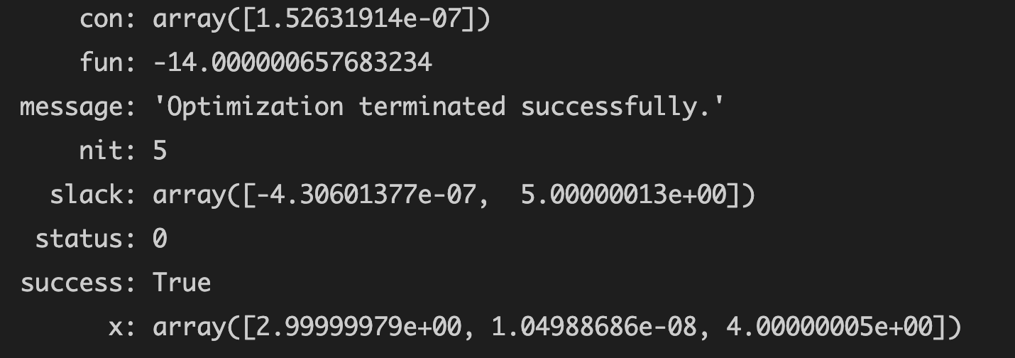
Operation results

• Optimal solution (minimum): - 14.000000657683234
• Corresponding to the optimal solution x n x_n xn​: array([2.99999979e+00, 1.04988686e-08, 4.00000005e+00])
  

Supplement - 1

If required 2 x 1 + 3 x 2 − 5 x 3 2x_1 + 3x_2 - 5x_3 2x1 + 3x2 − 5x3 max?

scipy.optimize.linprog can only find the minimum value of the objective function

If you need to find the maximum value of the objective function, you only need to change the parameter in the function to - c

Because when we find the maximum value of a function, we can find the minimum value of the objective function after the inverse (multiplied by - 1)
Multiply the minimum value by - 1 to get the maximum value
For example, the maximum value of function x1 + x2 is 2 (unknown in advance)
We can find the minimum value of - (x1 + x2) first
By solving, it is found that the minimum value of - (x1 + x2) is - 2
Then the maximum value is - 2 * - 1 = 2

Demo code

from scipy import optimize
import numpy as np

c = np.array([2,3,-5])

A_ub = np.array([[-2,5,-1],[1,3,1]])
b_ub = np.array([-10,12])

A_eq = np.array([[1,1,1]])
b_eq = np.array([7])

res = optimize.linprog(-c,A_ub,b_ub,A_eq,b_eq)
res

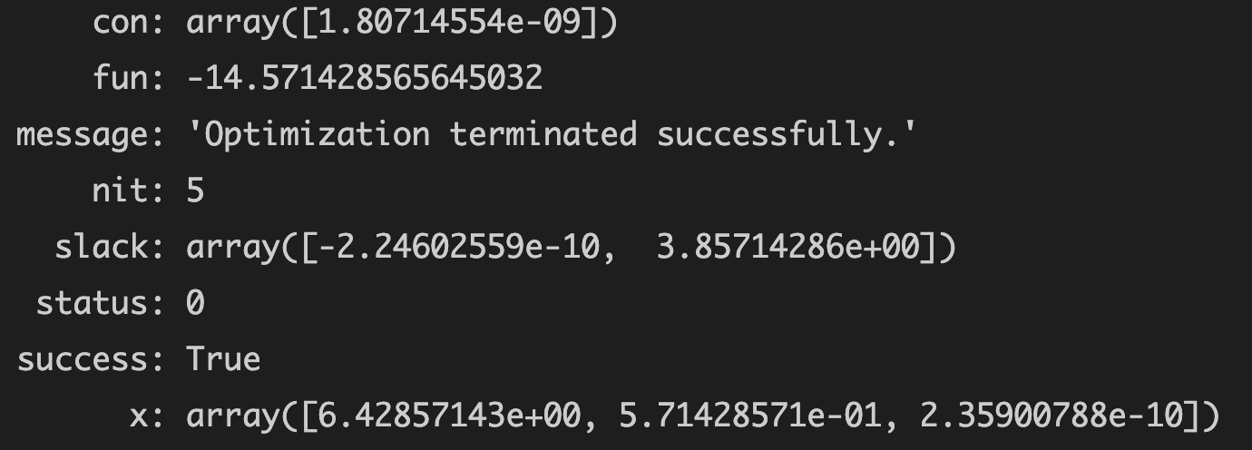
Operation results:

• The maximum value of the optimal solution is 14.571428565645032 (we seek the minimum value of - c, which is -14.571428565645032, then the maximum value of c is 14.571428565645032)
• Corresponding optimal solution x n x_n xn​: array([6.42857143e+00, 5.71428571e-01, 2.35900788e-10])
  

Supplement - 2

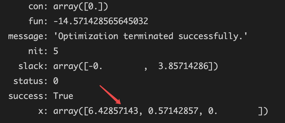
It can be found that the data in the final results are expressed in scientific notation

If scientific and technological law is not required for representation

Add code NP set_ Printoptions (suppress = true)

Demo code

from scipy import optimize
import numpy as np
np.set_printoptions(suppress=True)

c = np.array([2,3,-5])

A_ub = np.array([[-2,5,-1],[1,3,1]])
b_ub = np.array([-10,12])

A_eq = np.array([[1,1,1]])
b_eq = np.array([7])

res = optimize.linprog(-c,A_ub,b_ub,A_eq,b_eq)
res

Operation results

Supplement - 3

In the previous example, x n x_n The range of xn is x > = 0, belonging to SciPy optimize. Default value of the parameter bounds in linprog (0, None)

None: indicates unlimited

So if x n x_n xn# has a range limit, how to solve it?

The following questions:

m i n z = 2 x 1 + 3 x 2 − 5 x 3 s . t . = { x 1 + x 2 + x 3 = 7 2 x 1 − 5 x 2 + x 3 > = 10 x 1 + 3 x 2 + x 3 < = 12 0 < = x 1 < = 10 − 4 < = x 2 < = 10 1 < = x 3 < = 10 min z = 2x_1 + 3x_2 - 5x_3\\ s.t. = \begin{cases} x_1 + x_2 + x_3 = 7 \\ 2x_1 - 5x_2 + x_3 >= 10\\ x_1 + 3x_2 + x_3 <= 12\\ 0 < = x_1 <= 10 \\ -4 <= x_2 <= 10\\ 1 <= x_3 <= 10 \end{cases} minz=2x1​+3x2​−5x3​s.t.=⎩⎪⎪⎪⎪⎪⎪⎪⎪⎨⎪⎪⎪⎪⎪⎪⎪⎪⎧​x1​+x2​+x3​=72x1​−5x2​+x3​>=10x1​+3x2​+x3​<=120<=x1​<=10−4<=x2​<=101<=x3​<=10​

Solution: add a pair of unknowns x n x_n The restrictions of xn} are sufficient

Demo code

from scipy import optimize
import numpy as np

c = np.array([2,3,-5])

A_ub = np.array([[-2,5,-1],[1,3,1]])
b_ub = np.array([-10,12])

A_eq = np.array([[1,1,1]])
b_eq = np.array([7])

# Limit of unknowns
x1_bound = (0,10) # In tuple form
x2_bound = (-4,10)
x3_bound = (1,10)

res = optimize.linprog(-c,A_ub,b_ub,A_eq,b_eq,bounds=[x1_bound,x2_bound,x3_bound])
res

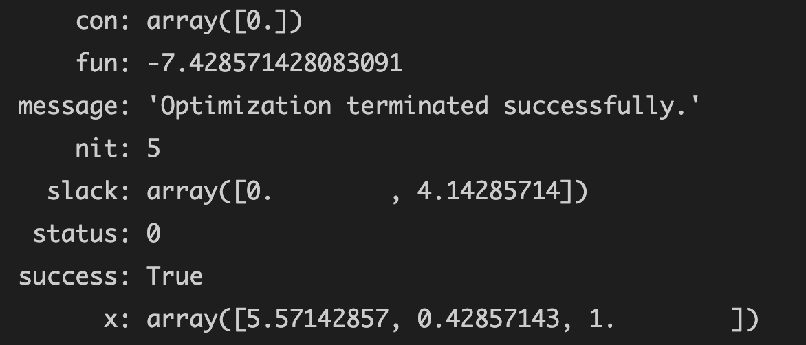
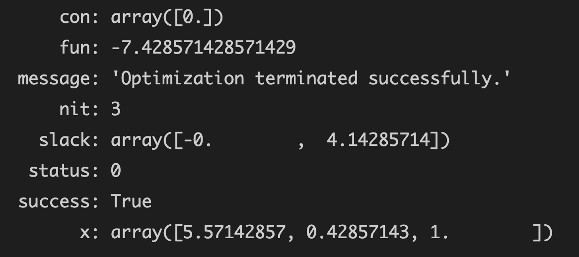
Operation results

• Optimal solution: 7.428571428083091 [here is the final fun result of max, which needs to be multiplied by - 1]
  

Supplement - 4

If higher accuracy is required, the parameter method can use revised simplex

Modify and compare with the topic in supplement - 3 (the optimal solution fun is slightly different)

Demo code

from scipy import optimize
import numpy as np

c = np.array([2,3,-5])

A_ub = np.array([[-2,5,-1],[1,3,1]])
b_ub = np.array([-10,12])

A_eq = np.array([[1,1,1]])
b_eq = np.array([7])

# Limit of unknowns
x1_bound = (0,10) # In tuple form
x2_bound = (-4,10)
x3_bound = (1,10)

res = optimize.linprog(-c,A_ub,b_ub,A_eq,b_eq,bounds=[x1_bound,x2_bound,x3_bound],method='revised simplex')
res

Operation results:

• Optimal solution: 7.428571428083091 [here is the final fun result of max, which needs to be multiplied by - 1]
  

Method 2: use the pump library

Preparatory knowledge

reference resources: https://blog.csdn.net/qq_20448859/article/details/72330362

1. LpProblem class

• LpProblem(name = 'NoName', sense=LpMinimize), constructor, used to construct an LP problem instance
  • Name specifies the problem name (for outputting information)
  • sense: one of LpMinimize or LpMaximize, which is used to specify whether the objective function is to find the maximum or minimum
• solve(solver=None, **kwargs): after adding constraints to LpProblem, the function is called to solve. If it is not for solving specific integer programming problems, solver generally uses the default.

2. LpVariable class

• LpVariable(name, lowBound=None, upBound=None, cat = 'Continuous', e=None), constructor, used to construct variables in LP problems

  • Name: Specifies the variable name
  • owBound and upBound are lower and upper bounds, which are negative infinity to positive infinity respectively by default,
  • cat is used to specify whether the variable is discrete (Integer,Binary) or continuous.

• dicts(name, indexs, lowBound=None, upBound=None, cat='Continuous', indexStart=[])
  It is used to construct variable dictionary, so that we don't have to create Lp variable instances one by one.

  • name specifies the prefix of all variables,
  • index is a list in which elements are used to form variable names. The last three parameters are the same as those in LbVariable.

3,lpSum(vector)

• Calculating the value of a sequence using lpSum is much faster than the ordinary sum function.

Note: it doesn't matter if you don't understand the concept. Temporarily skip the following example code and read the concept after understanding it

answer

m i n z = 2 x 1 + 3 x 2 − 5 x 3 s . t . = { x 1 + x 2 + x 3 = 7 2 x 1 − 5 x 2 + x 3 > = 10 x 1 + 3 x 2 + x 3 < = 12 x 1 , x 2 , x 3 > = 0 min z = 2x_1 + 3x_2 - 5x_3\\ s.t. = \begin{cases} x_1 + x_2 + x_3 = 7 \\ 2x_1 - 5x_2 + x_3 >= 10\\ x_1 + 3x_2 + x_3 <= 12\\ x_1,x_2,x_3 >= 0 \end{cases} minz=2x1​+3x2​−5x3​s.t.=⎩⎪⎪⎪⎨⎪⎪⎪⎧​x1​+x2​+x3​=72x1​−5x2​+x3​>=10x1​+3x2​+x3​<=12x1​,x2​,x3​>=0​

Demo code

import pulp as pp

# Parameter setting
c = [2,3,-5]        #Coefficient before unknown number of objective function

A_gq = [[2,-5,1]]   # A two-dimensional array of coefficient sets greater than or equal to the unknowns of the formula 
b_gq = [10]         # One dimensional array of values greater than or equal to the right of the formula

A_lq = [[1,3,1]]    # A two-dimensional array of coefficient sets less than or equal to the unknowns of the formula 
b_lq = [12]         # One dimensional array of values less than or equal to the right of the formula

A_eq = [[1,1,1]]    # A two-dimensional array of coefficient sets equal to the unknowns of the formula 
b_eq = [7]          # A one-dimensional array of values equal to the right of the formula

# The maximum minimization problem is determined. At present, the minimization problem is determined
m = pp.LpProblem(sense=pp.LpMinimize)

# Define three variables and put them in the list to generate x1 x2 x3
x = [pp.LpVariable(f'x{i}',lowBound=0) for i in [1,2,3]]

# Define the objective function and add the objective function to the problem to be solved 
# Generate 2*x1 + 3*x2 + (-5)*x3
m += pp.lpDot(c,x) # lpDot is used to calculate the dot product 

# Set comparison criteria
for i in range(len(A_gq)):# Greater than or equal to
    m += (pp.lpDot(A_gq[i],x) >= b_gq[i])

for i in range(len(A_lq)):# Less than or equal to
    m += (pp.lpDot(A_lq[i],x) <= b_lq[i])

for i in range(len(A_eq)):# be equal to
    m += (pp.lpDot(A_eq[i],x) == b_eq[i])

# solve
m.solve()

# Output results
print(f'Optimization results:{pp.value(m.objective)}')
print(f'Parameter value:{[pp.value(var) for var in x]}')

Operation results

Optimization results:-14.0
 Parameter value:[3.0, 0.0, 4.0]

Supplement - 1

Maximum if required

Just set the parameter sense in LpProblem to pp.LpMaximize

m = pp.LpProblem(sense=pp.LpMaximize)

m a x z = 2 x 1 + 3 x 2 − 5 x 3 s . t . = { x 1 + x 2 + x 3 = 7 2 x 1 − 5 x 2 + x 3 > = 10 x 1 + 3 x 2 + x 3 < = 12 x 1 , x 2 , x 3 > = 0 max z = 2x_1 + 3x_2 - 5x_3\\ s.t. = \begin{cases} x_1 + x_2 + x_3 = 7 \\ 2x_1 - 5x_2 + x_3 >= 10\\ x_1 + 3x_2 + x_3 <= 12\\ x_1,x_2,x_3 >= 0 \end{cases} maxz=2x1​+3x2​−5x3​s.t.=⎩⎪⎪⎪⎨⎪⎪⎪⎧​x1​+x2​+x3​=72x1​−5x2​+x3​>=10x1​+3x2​+x3​<=12x1​,x2​,x3​>=0​

Demo code

import pulp as pp

# Parameter setting
c = [2,3,-5]        #Coefficient before unknown number of objective function

A_gq = [[2,-5,1]]   # A two-dimensional array of coefficient sets greater than or equal to the unknowns of the formula 
b_gq = [10]         # One dimensional array of values greater than or equal to the right of the formula

A_lq = [[1,3,1]]    # A two-dimensional array of coefficient sets less than or equal to the unknowns of the formula 
b_lq = [12]         # One dimensional array of values less than or equal to the right of the formula

A_eq = [[1,1,1]]    # A two-dimensional array of coefficient sets equal to the unknowns of the formula 
b_eq = [7]          # A one-dimensional array of values equal to the right of the formula

# The maximum minimization problem is determined. At present, the maximization problem is determined
m = pp.LpProblem(sense=pp.LpMaximize)

# Define three variables and put them in the list to generate x1 x2 x3
x = [pp.LpVariable(f'x{i}',lowBound=0) for i in [1,2,3]]

# Define the objective function and add the objective function to the problem to be solved 
# Generate 2*x1 + 3*x2 + (-5)*x3
m += pp.lpDot(c,x) # lpDot is used to calculate the dot product 

# Set comparison criteria
for i in range(len(A_gq)):# Greater than or equal to
    m += (pp.lpDot(A_gq[i],x) >= b_gq[i])

for i in range(len(A_lq)):# Less than or equal to
    m += (pp.lpDot(A_lq[i],x) <= b_lq[i])

for i in range(len(A_eq)):# be equal to
    m += (pp.lpDot(A_eq[i],x) == b_eq[i])

# solve
m.solve()

# Output results
print(f'Optimization results:{pp.value(m.objective)}')
print(f'Parameter value:{[pp.value(var) for var in x]}')

Operation results

Optimization result: 14.57142851
 Parameter value:[6.4285714, 0.57142857, 0.0]

Supplement - 2

x n x_n xn# with restrictions:

m i n z = 2 x 1 + 3 x 2 − 5 x 3 s . t . = { x 1 + x 2 + x 3 = 7 2 x 1 − 5 x 2 + x 3 > = 10 x 1 + 3 x 2 + x 3 < = 12 0 < = x 1 < = 10 − 4 < = x 2 < = 10 1 < = x 3 < = 10 min z = 2x_1 + 3x_2 - 5x_3\\ s.t. = \begin{cases} x_1 + x_2 + x_3 = 7 \\ 2x_1 - 5x_2 + x_3 >= 10\\ x_1 + 3x_2 + x_3 <= 12\\ 0 < = x_1 <= 10 \\ -4 <= x_2 <= 10\\ 1 <= x_3 <= 10 \end{cases} minz=2x1​+3x2​−5x3​s.t.=⎩⎪⎪⎪⎪⎪⎪⎪⎪⎨⎪⎪⎪⎪⎪⎪⎪⎪⎧​x1​+x2​+x3​=72x1​−5x2​+x3​>=10x1​+3x2​+x3​<=120<=x1​<=10−4<=x2​<=101<=x3​<=10​

Add pair of unknowns x n x_n The limit of xn} is enough

bounds = [[0,10],[-4,10],[1,10]]#Variable range limit
x = [pp.LpVariable(f'x{i}',lowBound=bounds[i-1][0],upBound=bounds[i-1][1]) for i in [1,2,3]]

Demo code

import pulp as pp

# Parameter setting
c = [2,3,-5]        #Coefficient before unknown number of objective function

A_gq = [[2,-5,1]]   # A two-dimensional array of coefficient sets greater than or equal to the unknowns of the formula 
b_gq = [10]         # One dimensional array of values greater than or equal to the right of the formula

A_lq = [[1,3,1]]    # A two-dimensional array of coefficient sets less than or equal to the unknowns of the formula 
b_lq = [12]         # One dimensional array of values less than or equal to the right of the formula

A_eq = [[1,1,1]]    # A two-dimensional array of coefficient sets equal to the unknowns of the formula 
b_eq = [7]          # A one-dimensional array of values equal to the right of the formula

# The maximum minimization problem is determined. At present, the minimization problem is determined
m = pp.LpProblem(sense=pp.LpMaximize)

# Define three variables and put them in the list to generate x1 x2 x3
bounds = [[0,10],[-4,10],[1,10]]#Variable range limit
x = [pp.LpVariable(f'x{i}',lowBound=bounds[i-1][0],upBound=bounds[i-1][1]) for i in [1,2,3]]

# Define the objective function and add the objective function to the problem to be solved 
# Generate 2*x1 + 3*x2 + (-5)*x3
m += pp.lpDot(c,x) # lpDot is used to calculate the dot product 

# Set comparison criteria
for i in range(len(A_gq)):# Greater than or equal to
    m += (pp.lpDot(A_gq[i],x) >= b_gq[i])

for i in range(len(A_lq)):# Less than or equal to
    m += (pp.lpDot(A_lq[i],x) <= b_lq[i])

for i in range(len(A_eq)):# be equal to
    m += (pp.lpDot(A_eq[i],x) == b_eq[i])

# solve
m.solve()

# Output results
print(f'Optimization results:{pp.value(m.objective)}')
print(f'Parameter value:{[pp.value(var) for var in x]}')

Operation results

Optimization result: 7.4285714899999995
 Parameter value:[5.5714286, 0.42857143, 1.0]

Of course, there is another way to x n x_n xn ， the restricted form is rewritten into a general linear programming (the unknowns are placed on the left)

m i n z = 2 x 1 + 3 x 2 − 5 x 3 s . t . = { x 1 + x 2 + x 3 = 7 2 x 1 − 5 x 2 + x 3 > = 10 x 1 + 3 x 2 + x 3 < = 12 x 1 > = 0 x 1 < = 10 x 2 > = − 4 x 2 < = 10 x 3 > = 1 x 3 < = 10 min z = 2x_1 + 3x_2 - 5x_3\\ s.t. = \begin{cases} x_1 + x_2 + x_3 = 7 \\ 2x_1 - 5x_2 + x_3 >= 10\\ x_1 + 3x_2 + x_3 <= 12\\ x_1 >= 0 \\ x_1 <= 10\\ x_2 >= -4 \\ x_2 <= 10\\ x_3 >= 1\\ x_3 <= 10 \end{cases} minz=2x1​+3x2​−5x3​s.t.=⎩⎪⎪⎪⎪⎪⎪⎪⎪⎪⎪⎪⎪⎪⎪⎪⎨⎪⎪⎪⎪⎪⎪⎪⎪⎪⎪⎪⎪⎪⎪⎪⎧​x1​+x2​+x3​=72x1​−5x2​+x3​>=10x1​+3x2​+x3​<=12x1​>=0x1​<=10x2​>=−4x2​<=10x3​>=1x3​<=10​

You only need to modify the parameter settings (add a set of coefficients before several unknowns)

A_gq = [[2,-5,1],[1,0,0],[0,1,0],[0,0,1]]   # A two-dimensional array of coefficient sets greater than or equal to the unknowns of the formula 
b_gq = [10,0,-4,1]         # One dimensional array of values greater than or equal to the right of the formula

A_lq = [[1,3,1],[1,0,0],[0,1,0],[0,0,1]]    # A two-dimensional array of coefficient sets less than or equal to the unknowns of the formula 
b_lq = [12,10,10,10]         # One dimensional array of values less than or equal to the right of the formula

Demo code

import pulp as pp

# Parameter setting
c = [2,3,-5]        #Coefficient before unknown number of objective function

A_gq = [[2,-5,1],[1,0,0],[0,1,0],[0,0,1]]   # A two-dimensional array of coefficient sets greater than or equal to the unknowns of the formula 
b_gq = [10,0,-4,1]         # One dimensional array of values greater than or equal to the right of the formula

A_lq = [[1,3,1],[1,0,0],[0,1,0],[0,0,1]]    # A two-dimensional array of coefficient sets less than or equal to the unknowns of the formula 
b_lq = [12,10,10,10]         # One dimensional array of values less than or equal to the right of the formula

A_eq = [[1,1,1]]    # A two-dimensional array of coefficient sets equal to the unknowns of the formula 
b_eq = [7]          # A one-dimensional array of values equal to the right of the formula

# The maximum minimization problem is determined. At present, the maximization problem is determined
m = pp.LpProblem(sense=pp.LpMaximize)

# Define three variables and put them in the list to generate x1 x2 x3
x = [pp.LpVariable(f'x{i}') for i in [1,2,3]]

# Define the objective function and add the objective function to the problem to be solved 
# Generate 2*x1 + 3*x2 + (-5)*x3
m += pp.lpDot(c,x) # lpDot is used to calculate the dot product 

# Set comparison criteria
for i in range(len(A_gq)):# Greater than or equal to
    m += (pp.lpDot(A_gq[i],x) >= b_gq[i])

for i in range(len(A_lq)):# Less than or equal to
    m += (pp.lpDot(A_lq[i],x) <= b_lq[i])

for i in range(len(A_eq)):# be equal to
    m += (pp.lpDot(A_eq[i],x) == b_eq[i])

# solve
m.solve()

# Output results
print(f'Optimization results:{pp.value(m.objective)}')
print(f'Parameter value:{[pp.value(var) for var in x]}')

Operation results:

Optimization result: 7.4285714899999995
 Parameter value:[5.5714286, 0.42857143, 1.0]