catalogue
1 data analysis function library
1.2 functions for random data analysis
1.3 functions for correlation analysis
2. Polynomial function library
2.1} four operations of polynomials
2.2 derivation, root and evaluation of polynomials
2.4 solutions of linear differential equations
3. Nonlinear function analysis and numerical integration of function
3.1 nonlinear function analysis
3.2 numerical integration of function
1 data analysis function library
1.1 basic data analysis
Basic data processing functions are performed by column:
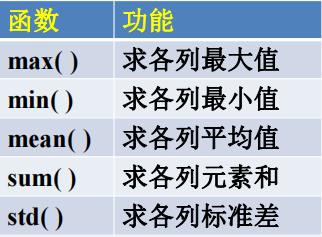
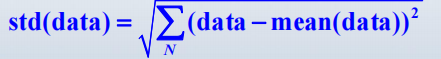
The standard deviation is N in the column
The square sum of the difference between the elements and the average value of the column.
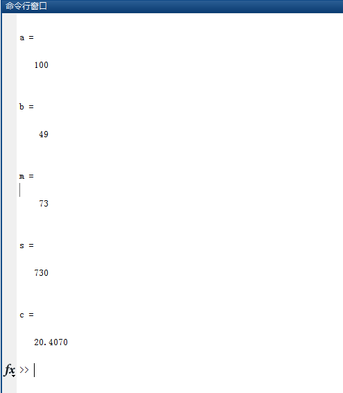
%Example 1.1
data=[49 99 100 63 63 55 56 89 96 60]';
a=max(data)
b=min(data)
m=mean(data)
s=sum(data)
c=std(data)
1.2 functions for random data analysis
rand(m,n) :
Generated at 0
~
Between 1
uniform distribution
of
m
OK
n
Column random number matrix.
randn(m,n) :
produce
Normal distribution
of
m
OK
n
Column random
Number matrix, the mean value is 0 and the standard deviation is 1.
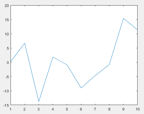
%Example 1.2
y= 5*(randn(1,10)-.5)
plot(y)
1.3 functions for correlation analysis
corrcoef(x,y):
Calculate two vectors
x
,
y
Correlation coefficient of
cov(x,y):
calculation
x
,
y
Covariance matrix of
%Example 1.3
x= rand(1,10)
y= rand(1,10)
corrcoef(x,y)
%result
x =

    0.7060    0.0318    0.2769    0.0462    0.0971    0.8235    0.6948    0.3171    0.9502    0.0344


y =

    0.4387    0.3816    0.7655    0.7952    0.1869    0.4898    0.4456    0.6463    0.7094    0.7547


ans =

    1.0000   -0.0403
   -0.0403    1.0000
2. Polynomial function library
2.1} four operations of polynomials
(1) Representation of polynomials
Expressed by the coefficient vector before each power, from high to low.

a=[a(1), a(2),...,a(
n
), a(
n
+1)]
be careful
: zero coefficient cannot be omitted.
a=[1, 2, 0, 1]
b=[1, 2, 1]
(2) Polynomial operation
♥
Polynomial addition:
a+b
Note:
The length must be the same, and the shorter one is
front
Complete with "0".
♥
Polynomial multiplication:
conv(a,b)
♥
Polynomial division:
[q,r]=deconv(a,b)
q
: quotient
r
: remainder formula
be careful
:
a
It's a molecule,
b
Is the denominator. The first digit of the denominator coefficient vector cannot be zero.
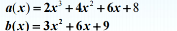
%Example 2.1
a=[2, 4, 6, 8]
b=[3, 6, 9]
c=a+[0, b]
d=conv(a,b) [q,r]=deconv(d,a) [q,r]=deconv(a,b)
%result
c =

     2     7    12    17


d =

     6    24    60    96   102    72


q =

     3     6     9


r =

     0     0     0     0     0     0


q =

    0.6667         0


r =

     0     0     0     8
2.2 derivation, root and evaluation of polynomials
♥
Polynomial derivation:
polyder(a)
♥
Polynomial root:
roots(a)
♥
Finding polynomial coefficients from roots:
poly(a)
♥
Polynomial evaluation:
polyval(a,xv)
Give polynomial a
Arguments in
x
Assign value
xv
.
Example 2.2
%Example 2.2
a=[2, 4, 6, 8]
a1=polyder(a)
a2=roots(a)
a3=poly(a2)
a4=polyval(a,1)
%result
a =

     2     4     6     8


a1 =

     6     8     6


a2 =

  -1.6506 + 0.0000i
  -0.1747 + 1.5469i
  -0.1747 - 1.5469i


a3 =

    1.0000    2.0000    3.0000    4.0000


a4 =

    20
2.3 polynomial fitting
fitting
: find a mathematical expression based on a set of known data.
Fitting method
: to minimize the variance, the least square method is applied.
p=polyfit(x,y,n)
x
,
y
Is known
N
A data point coordinate vector,
n
Is fitting
Polynomial degree of,
p
Is the calculated polynomial coefficient vector.
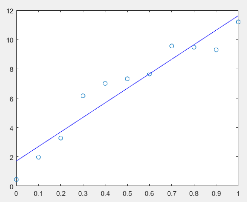
Example 2.3
At 11 points(
x=0:0.1:1
)The value measured on the is
y=[0.447,1.978,3.28,6.16,7.01,7.32,7.66,
9.56,9.48,9.30,11.2]
Try the least square method to find the fitting curve.
%Example 2.3
x=(0:0.1:1)
y=[0.447,1.978,3.28,6.16,7.01,7.32,7.66,9.56,9.48,9.30,11.2]
a1=polyfit(x,y,1);
xi=x
yi1=polyval(a1,xi);
plot(x,y,'o',xi,yi1,'b')
2.4 solutions of linear differential equations
First use
Laplace transform
Transform linear ordinary differential equations
by
algebraic equation
, the expression of the response is
s
Rational fraction of.
(1) Partial fraction expansion
(2) Inverse transformation
(assuming denominator is higher than numerator order)
[r,p,k]=residue(b,a)
y(t)=r(1)*exp(p(1)*t)+ r(2)*exp(p(2)*t)+
⋯

3. Nonlinear function analysis and numerical integration of function
3.1 nonlinear function analysis
Draw function curve
fplot
(
'
Function name
'
, [initial value, final value])
Finding function extremum
fmin
(
'
Function name
'
, initial value, final value)
Find the zero of the function
fzero
(
'
Function name
'
, initial guess value)
3.2 numerical integration of function
Definite integral subroutine
quad
(
'
Function name
'
, initial value, final value)
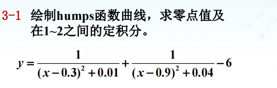
function y=humps(x)
y= 1./((x-0.3).^2+0.01)+1./((x-.9).^2+.04)-6;
fplot('humps',[0, 2]),grid
z=fzero('humps',1)
s=quad('humps',1,2) 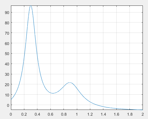
%result
z =

    1.2995


s =

   -0.5321