The following examples are the official examples of MathWorks. I have translated and sorted out the relevant knowledge points and recorded the learning notes.
Original link: https://ww2.mathworks.cn/help/nav/ref/referencepathfrenet.html
Generate Alternative Trajectories for Reference Path
Use Frenet coordinates to generate alternative tracks for the reference path. Specify different initial and terminal states for tracks. Adjust the state according to the generated trajectory.
Generate a reference path from the collection of waypoints, and create an object of trajectoryGeneratorFrenet from the reference path.
waypoints = [0 0;50 20;100 0;150 10];
%Create a collection of path points

refPath = referencePathFrenet(waypoints);
%Through function referencePathFrenet A smooth curve based on the set of path points is generated refPath

connector = trajectoryGeneratorFrenet(refPath);
%Through function trajectoryGeneratorFrenet Generation based refPath A track of
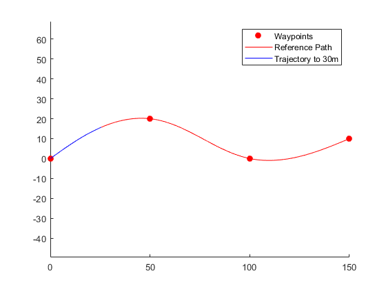
A 5-second trajectory is generated between the origin of the path and the point 30 meters below the path as the initial state and final state of Frenet.
initState = [0 0 0 0 0 0];  % [S ds ddS L dL ddL] Initial state

termState = [30 0 0 0 0 0]; % [S ds ddS L dL ddL] Final state

[~,trajGlobal] = connect(connector,initState,termState,5);
%Among them~Represents the parameter that ignores the first output, and then passes connect The function connects the initial and final states, and 5 represents the time interval 5 s.
Displays the track in global coordinates.
show(refPath);
%Functions that display paths

hold on

axis equal
%The scale of horizontal and vertical coordinates is equal

plot(trajGlobal.Trajectory(:,1),trajGlobal.Trajectory(:,2),'b')
%Draw a picture

legend(["Waypoints","Reference Path","Trajectory to 30m"])
%Set legend
The results are as follows:
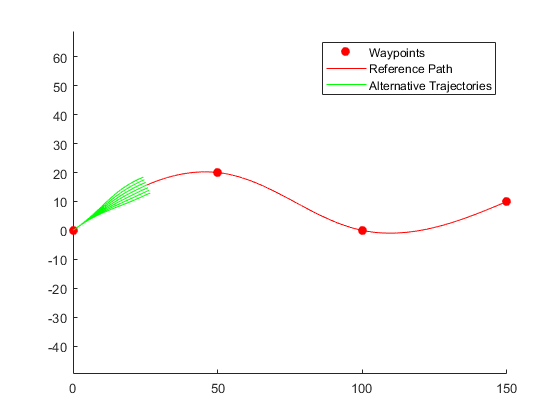
Create a terminal state matrix with a lateral deviation of - 3m to 3m. Generate a trajectory that covers the same arc length in 10 seconds but deviates laterally from the reference path. Displays the new alternate path. To put it bluntly, the terminal state is changed into several, and the lateral deviation is limited.
termStateDeviated = termState + ([-3:3]' * [0 0 0 1 0 0]);
[~,trajGlobal] = connect(connector,initState,termStateDeviated,5);

clf
show(refPath);
hold on
axis equal
for i = 1:length(trajGlobal)
    plot(trajGlobal(i).Trajectory(:,1),trajGlobal(i).Trajectory(:,2),'g')
end
legend(["Waypoints","Reference Path","Alternative Trajectories"])
hold off
The results are as follows:
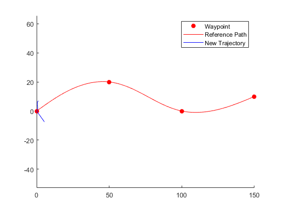
Specify a new terminal state (the final state and time interval have changed) to generate a new track. This trajectory is undesirable (unreasonable) because it requires reverse motion to achieve a lateral speed of 10 meters / second.
newTermState = [5 10 0 5 0 0];
[~,newTrajGlobal] = connect(connector,initState,newTermState,3);

clf
show(refPath);
hold on
axis equal
plot(newTrajGlobal.Trajectory(:,1),newTrajGlobal.Trajectory(:,2),'b');
legend(["Waypoint","Reference Path","New Trajectory"])
hold off
The results are as follows:
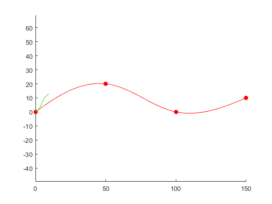
The restriction on the longitudinal state is relaxed by specifying the arc length NaN. Generate and display the track again. The new position shows a good alternative trajectory that deviates from the reference path.
relaxedTermState = [NaN 10 0 5 0 0];
%NAN Not a Number Represents a null value, relaxing the restriction on arc length

[~,trajGlobalRelaxed] = connect(connector,initState,relaxedTermState,3);
%The time interval is set to 3 s

clf
%Clear old image

show(refPath);
%Show reference tracks

hold on

axis equal

plot(trajGlobalRelaxed.Trajectory(:,1),trajGlobalRelaxed.Trajectory(:,2),'g');
%Draw a picture

hold off
The results are as follows:
The functions used in the above examples are described as follows:
1,referencePathFrenet
The corresponding smooth reference path is generated through the path points.
referencePathFrenet passes through a group with [x, y] or [x, y] θ] The given path points fit a smooth, segmented and continuous curve. After fitting, the path points along the curve are expressed as [x y theta kappa dkappa s], where:
X, y and theta - a two-dimensional matrix, expressed in the global coordinate system, x, y in meters and theta in radians
kappa -- curvature, or reciprocal of radius, in meters
dkappa -- derivative of curvature to arc length, unit: M / s
s -- arc length, or the distance from the path to the path origin, in meters
Using this object, the trajectory is converted between the global coordinate system and Frenet coordinate system, the state is interpolated along the path based on the arc length, and the nearest point on the path is queried from the global state.
Object represents the Frenet state as a vector of the form [S dS ddS L dL ddL], where s is the arc length and l is the vertical deviation from the direction of the reference path. The derivative of S is relative to time. The derivative of L is related to the arc length s.
refPathObj = referencePathFrenet(waypoints)

refPathObj = referencePathFrenet(waypoints,'DiscretizationDistance',discretionDist)
%The difference between the two syntax is that the second syntax can customize the distance between path points.
%The second method uses interpolation path points to speed up the conversion function frenet2global and Global2Frenet Performance.
%Smaller discretization distance can improve accuracy at the expense of memory and computational efficiency.
| function | describe |
|---|---|
| closestPoint | Find the nearest point on the reference path of the global point |
| frenet2global | Convert Frenet state to global state |
| global2frenet | Convert global state to Frenet state |
| interpolate | Interpolates the reference path at a given arc length |
| show | Show reference path in Figure |
2,trajectoryGeneratorFrenet
Used to find the optimal trajectory along the reference path.
This function uses fourth-order or fifth-order polynomials based on a given reference path to generate a turnover trajectory. Each track defines a motion between Frenet states within a specified time span.
Frenet states describe their position, velocity, and acceleration at different points in time relative to a static reference path specified as an object created by the function referencePathFrenet.
Object represents the Frenet state as a vector of the form [S dS ddS L dL ddL], where s is the arc length and l is the vertical deviation from the direction of the reference path. The derivative of S is relative to time. The derivative of L is related to the arc length s.
To generate alternative tracks, assign the initial and terminal frenet states for a given time span to the connect objective function.
connectorFrenet = trajectoryGeneratorFrenet(refPath)
%Created by this function from Frenet Initial state to Frenet Trajectories between final states,
%Is based on function referencePathFrenet Created reference path refPath of
%refPath Input parameter settings ReferencePath Properties.

connectorFrenet = trajectoryGeneratorFrenet(refPath,'TimeResolution',timeValue)
%Specifies the time interval for discretization. timeValue Parameter setting TimeResolution Properties.
| function | describe |
|---|---|
| connect | Connect the initial Frenet state and the final Frenet state |
3,connect
Used to connect the initial Frenet state and the final Frenet state.
frenetTrajectory = connect(connectorFrenet,initialState,terminalState,timeSpan)
%Sets the specified initial value in seconds over a period of time Frenet Status connects to the specified terminal status.
%This objective function supports 1 pair N,N For 1 or N yes N Paired track connections.

[___,globalTrajectory] = connect(___)
%In addition to returning all parameters in the previous syntax, it also returns tracks in global coordinates.