Note:

• Although the document is very comprehensive, this article is mainly for quick completion in one day, so please forgive me for the shortcomings.
• The code is based on matlab terminal called by vscode/py 3.6

Basic mathematical operation and matrix operation

Basic grammar

variable

• No declaration required
• Assign a value to a variable with =

Variable name

• Variable names are case sensitive (I don't know if it's because of windows)
• Variable names can only be [0~9,a~z,A~z,] And the variable name cannot start with a number
• Reserved variables are not suitable for variable names
  • Use the iskeyword command to view program keywords, which are not allowed to be used as variable names

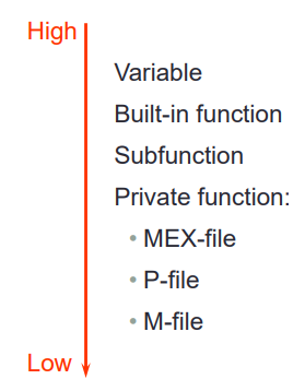
Variable names should not override built-in function names

In MATLAB, the calling priority of variable is higher than that of function, so the variable name should not overwrite the built-in function

For example:

cos = 'changqingaas';
cos(8)
% disp(['ans is ', num2str(ans)])
clear; % If a function is overwritten by a variable name,Then call clear <Variable name>You can unbind the variable name on the function name
cos(8)
% disp(['ans is ', num2str(ans)])

Note: clear is a dangerous command, because if no parameters are added after the command, it means to clear all variables in the current workspace

Output:

ans =

    'n'


ans =

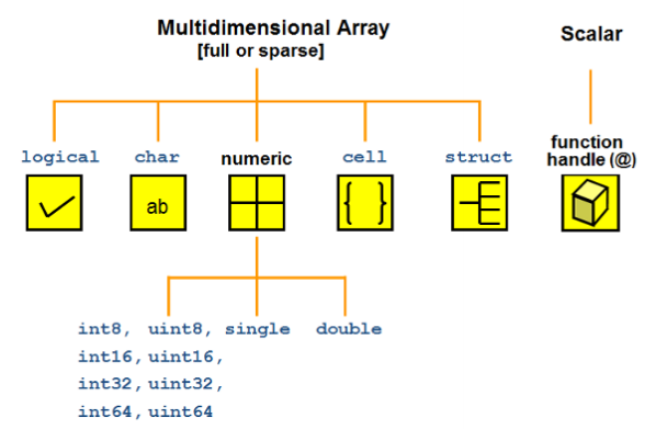
   -0.1455

Variable type

logical,char,numeric,cell,struct and their array or matrix

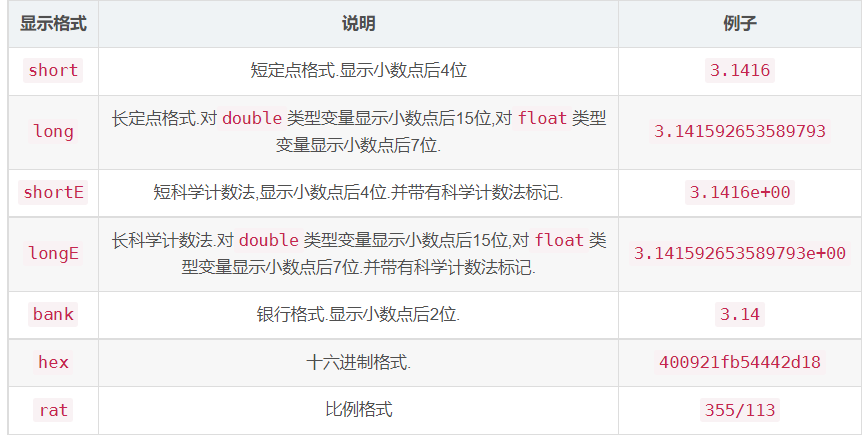
Display format of numeric variables

Numeric variable, which is stored in the form of double by default

You can change the display format of numeric variables through format < Display Format >

MATLAB command line

• Use end of line; Suppress output:
  • Use after one line of command; Suppress the output, otherwise the operation result will be displayed on the terminal
• |Command | function | operation result| | -—- | --------------- | --------------- | |clc | clear the output of the terminal || |Clear | clear all variables in the current workspace by default || |who | displays all variables in the workspace in a simplified format | your variables are: ans | |whos | display all variables in the workspace in complex format | name size bytes class attributes ans 1x1 8 double | |which | view the location of the source code file of the built-in function. Combined with the edit command, you can view the source code of the built-in function|

Use MATLAB for digital operation

Calculate mathematical expressions using MATLAB

• After the mathematical expression is calculated, its value is stored in the variable ans
• log indicates ln
• exp(x) means e^x

MATLAB built-in mathematical function

• MATLAB built-in arithmetic operation function
  • Basic operation:
    • Plus: +, sum,cumsum,movsum
    • Minus: -, diff
    • Multiply by:. *, *, prod,cumprod
    • Except:. /,. \, /\
    • Power: ^^
  • Modular operation: mod,rem,idivide,ceil,fix,floor,round
• MATLAB built-in trigonometric operation function
  • Sine: sin,sind,sinpi,asin,asind,sinh,asinh
  • Cosine: cos,cosd,cospi,acos,acosd,cosh,acosh
  • Tangent: tan,tand,atan,atand,atan2,atan2d,tanh,atanh
  • Cosecant: csc,cscd,acsc,acscd,csch,acsch
  • Secant: sec,secd,asec,asecd,sech,asech
  • cot,cotd,acot,acotd,coth,acoth
  • Bevel: hypot
  • Conversion: deg2rad,rad2deg,cart2pol,cart2sph,pol2cart,sph2cart
• Built in exponential logarithm function of MATLAB:
  • exp,expm1,log,log10,log1p,log2,nextpow2,nthroot,pow2,reallog,realpow,realsqrt,sqr
• Complex functions built in MATLAB:
  • abs,angle,complex,conj,cplxpair,i,imag,isreal,j,real,sign,unwrap

Matrix operation using MATLAB

Definition matrix

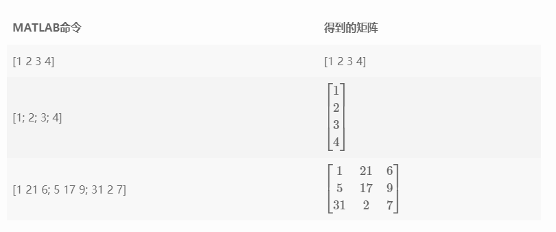
Input matrix to terminal

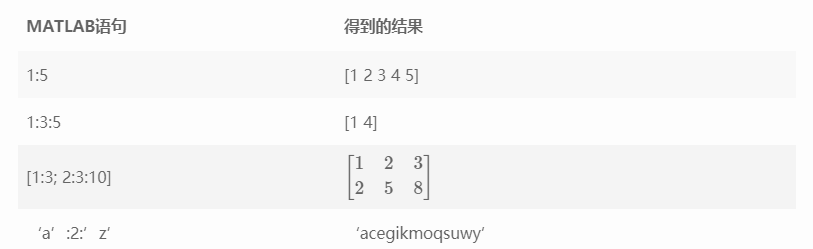
In MATLAB, use [] to enclose the matrix content to be input, use spaces or commas to separate variables in the line, and use; Separate each line

Create vectors using colon operators

Using colon operator: you can create a long vector with the following syntax:

For example:

Define special matrix

Index of matrix

• The matrix in MATLAB is stored in column order And the index subscript starts from 1
• There are two indexing methods for matrices: one-dimensional indexing and two-dimensional indexing For a general matrix, the index order is as follows: \ begin{bmatrix} 1 or (1,1) & 4 or (1,2) & 7 or (1,3) \ \ 2 or (2,1) & 5 or (2,2) & 8 or (2,3) \ \ 3 or (3,1) & 6 or (3,2) & 9 or (3,3) \ end {bMatrix}
• The index of matrix can use colon:, which means to select all rows or columns
• The index of the matrix can be one or two vectors, representing all rows or columns in the selected vector| The result of the original matrix | index | ------------------------------------------------------------------------------------------------------| \ begin {bmatrix} 1 & 2 & 3 \ 4 & 5 & 6\ 7 & 8 & 9 \end{bmatrix}\begin{bmatrix} 1 & 2 & 3 \ 4 & 5 & 6\ 7 & 8 & 9 \end{bmatrix}\begin{bmatrix} 1 & 2 & 3 \ 4 & 5 & 6\ 7 & 8 & 9 \end{bmatrix}\begin{bmatrix} 1 & 4 \ 7 & 2\end{bmatrix}\begin{bmatrix} 1 & 2 & 3 \ 4 & 5 & 6\ 7 & 8 & 9 \end{bmatrix}\begin{bmatrix} 1 & 2 & 3 \ 4 & 5 & 6\ 7 & 8 & 9 \end {bmatrix}\begin{bmatrix} 1 & 2 & 3 \ 4 & 5 & 6 \end{bmatrix}\begin{bmatrix} 1 & 2 & 3 \ 4 & 5 & 6\ 7 & 8 & 9 \end{bmatrix}\begin{bmatrix} 1 & 2 \ 7 & 8 \end{bmatrix}

Matrix operation

Operator of operation matrix

Function of operation matrix

For the following matrix

A=\begin{bmatrix} 1 & 2 & 3 \\ 0 & 5 & 6 \\ 7 & 0 & 9 \end{bmatrix}

Operate to demonstrate common functions of the operation matrix

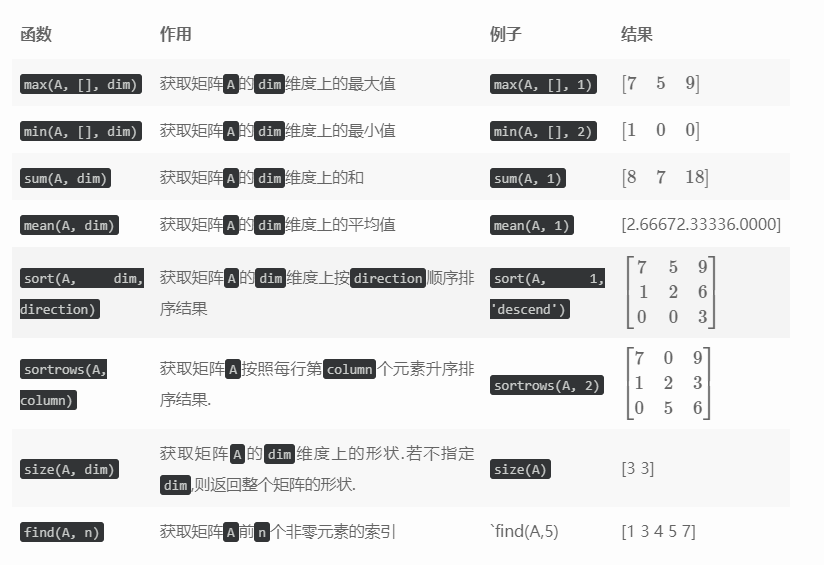
For the above functions, all parameters are optional except the first parameter

Structured programming and function definition

Structured programming

Process control statements and logical operators

All the above loops and conditional statements should be closed with end at the end

MATLAB also has the following logical operators:

Example of process control statement

if statement:

if condition1
	statement1
elseif condition2
	statement2
else 
	statement3
end

switch Statements

switch expression
    case value1
        statement1
    case value2
        statement2
    otherwise 
        statement
end

while statement

while expression
	statement
end

for statement

for variable = start:increment:end
	commands
end

break statement

x = 2; k = 0; error = inf;
error_threshold = 1e-32;

while error > error_threshold

    if k > 100
        break
    end

    x = x - sin(x) / cos(x);
    error = abs(x - pi);
    k = k + 1;
end

Try to pre allocate memory space when using circular statements

Problems needing attention when writing scripts

A statement should be added at the beginning of the script to empty the workspace

At the beginning of each script, the following statement should be added to empty the workspace cache and traces of previous program operation:

clear all	% Clear variables in workspace memory
close all 	% Close the image drawn by the previous program
clc			% Output of the program at the terminal before emptying

Semicolon shall be added after operation and assignment statement; Suppress output

Semicolons should be added to all operations and assignment statements; Suppress the output. If you need to output a variable to the terminal, you should call the disp method

Use ellipsis Splicing multiline statements

In MATLAB, ellipsis Multiple lines of statements can be spliced into one line, and the flexible use of this statement can improve the readability of the code

function

Similar to scripts, functions can be stored in function names m file can also be defined in memory in the form of function handle

View built-in functions

We can use the which command to view the location of the source code file of the built-in function. Combined with the edit command, we can view the source code of the built-in function

Run the following statement to open the source file of MATLAB's built-in mean function:

edit(which('mean.m'))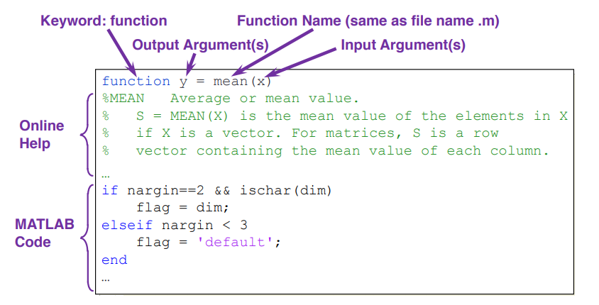

In function name m file form definition function

The format of the function defined in the MATLAB file is as follows:

function [Output variable name] = Function name(Enter variable name) 
% Documentation of functions

function code

• Function is a keyword that declares that a function is saved in the file
• Input variables and output variables are not necessary. Functions can have neither input variables nor output variables
• Function name should be the same as m file name is the same and does not contain special characters (preferably Chinese)

MATLAB built-in function parameters

MATLAB does not provide syntax for specifying default parameter values and function overloading in other high-level languages, but the flexible use of the above built-in function parameters can realize specifying default parameter values and method overloading to a certain extent:

MATLAB function definition example 1

The surface program is used to calculate the displacement in the free fall movement: x = x_{0} + v_{0}t + \frac{1}{2} g t^2

function x = freebody(x0,v0,t)
% calculation of free falling
% x0: initial displacement in m
% v0: initial velocity in m/sec
% t: the elapsed time in sec
% x: the depth of falling in m
x = x0 + v0.*t + 1/2*9.8*t.*t;

This function demonstrates a MATLAB programming skill: try to use it when calculating multiplication* Not *, because the former is available not only when the parameter t is scalar, but also when the variable t is vector or matrix

freebody(0, 0, 2)			% Get 19.6000
freebody(0, 0, [0 1 2 3])	% obtain [0 4.9000 19.6000 44.1000]
freebody(0, 0, [0 1; 2 3])	% obtain [0 4.9000; 19.6000 44.1000]

MATLAB function definition example 2

The following function realizes the conversion from Fahrenheit temperature to Celsius temperature. This function can identify the number of input samples to be converted. When the number of input samples to be converted is 0, exit the function

function F2C()
while 1
    F_degree = input('tempreature in Fahrenheit: ', 's');
    F_degree = str2num(F_degree);
    if isempty(F_degree)
        return
    end
    C_degree = (F_degree-32)*5/9;
    disp(['tempreature in Celsius: ' num2str(C_degree)])
end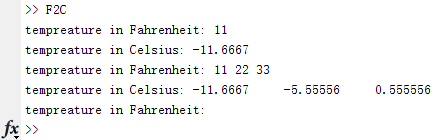

Define a function as a function handle

We can also define a function in the form of a function handle, which is closer to the mathematical function definition. Its syntax is as follows:

Function handle  = @(Input variable) Output variable 

This method can be called directly through the function handle

f = @(x) exp(-2*x);
x = 0:0.1:2;
plot(x, f(x));

Data type and file reading and writing

data type

The main data types in MATLAB are as follows:

Numeric type

The numerical types supported by MATLAB are shown in the following table:

The value type of. double can be converted to the value type of other variables in MATLAB by default

n = 3;
class(n)	 

n = int8(3);
class(n)	 

Output:

ans =
    'double'
ans =
    'int8'

String type (char)

In MATLAB, the string type is defined by a pair of single quotation marks' wrapping a text Standard ASCII characters can be converted to corresponding ASCII codes

s1 = 'h';
uint16(s1)	% Get 104

Strings are stored in memory in the form of character matrix, which can be indexed and assigned:

str1 = 'hello';
str2 = 'world';

str3 = [str1 str2];
size(str3)		% obtain [1 10]

str4 = [str1; str2];
size(str4)		% obtain [2 5]

str = 'aardvark';
'a' == str				% obtain [1 1 0 0 0 1 0 0]
str(str == 'a') = 'Z'	% obtain 'ZZrdvZrk'

Structure

In MATLAB, the structure is a key value pair

Basic use of structure

• Similar to most programming languages, MATLAB uses To access fields in the structure:

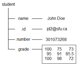
student.name = 'John Doe';
student.id = 'jdo2@sfu.ca';
student.number = 301073268;
student.grade = [100, 75, 73; ...
                 95, 91, 85.5; ...
                 100, 98, 72];
student

Using subscript expressions on the structure list can expand or reduce the structure list

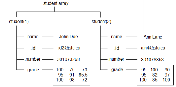
student.name = 'John Doe';
student.id = 'jdo2@sfu.ca';
student.number = 301073268;
student.grade = [100, 75, 73; 95, 91, 85.5; 100, 98, 72];

student

student(2).name = 'Ann Lane';
student(2).id = 'aln4@sfu.ca';
student(2).number = 301078853;
student(2).grade = [95 100 90; 95 82 97; 100 85 100];

student(1) = [] % delete student First item in the list

Structures can be cascaded, that is, the value of fields in structures can also be structures:

A = struct('data', [3 4 7; 8 0 1], ...
'nest', struct('testnum', 'Test 1', ...
'xdata', [4 2 8], ...
'ydata', [7 1 6]));
A(2).data = [9 3 2; 7 6 5];
A(2).nest.testnum = 'Test 2';
A(2).nest.xdata = [3 4 2];
A(2).nest.ydata = [5 0 9];

A

Common functions of structures

Cell array

In MATLAB, cell array is a data structure that can accommodate different types of elements, similar to the list in Python language

Basic use of cell array

Use {} to define a cell array like a matrix:

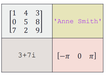
A = { [1 4 3; 0 5 8; 7 2 9]		'Anne Smith' ;...
3+7i		-pi:pi:pi}

A(1,1)={[1 4 3; 0 5 8; 7 2 9]};
A(1,2)={'Anne Smith'};
A(2,1)={3+7i};
A(2,2)={-pi:pi:pi};

A{1,1}=[1 4 3; 0 5 8; 7 2 9];
A{1,2}='Anne Smith';
A{2,1}=3+7i;
A{2,2}=-pi:pi:pi;
A

The above three methods are equivalent. The second method uses unit index assignment and the third method uses content index assignment

• There are two ways to access data in a cell array: the cell index () and the content index {} Because the subset of cell array is still cell array, it is necessary to indicate whether we want to access a sub cell array or the content in the corresponding area of cell array in the use of indexer content
  • Using the cell index (), we get an array of sub cells
    • Using the content index {}, we get the content in the corresponding area of the cell array

Common functions of cell array

Common functions of cell array

The mat2cell function can specify the size of each cell in the cell array during conversion

a = magic(3)

b = num2cell(a)
% obtain
% [8] [1] [6]
% [3] [5] [7]
% [4] [9] [2]

c = mat2cell(a, [1 2], [2, 1])
% obtain
% [1x2 double] [6]
% [2x2 double] [2x1 double]

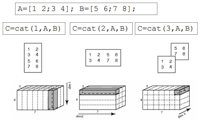
High dimensional cell array

A three-dimensional cell array can have three dimensions: row, column and layer When indexing cellular arrays, the order of priority from high to low is: row → column → layer

Using cat function, you can splice the cell array on the specified dimension

Function for judging variable data type

The following functions can judge the type of variables:

File reading and writing

The supported file types are as follows:

Read and write data in MATLAB format

The data in MATLAB workspace can be expressed in * The mat format is saved in a file Use the save function to save the data into the file, and use the load function to read the data from the file

• save The syntax of the function is as follows:
  • save(filename,variables) saves the variables into a file in binary form
  • save(filename,variables,'-ascii') saves the variables to a file as text
• load The syntax of the function is as follows:
  • load(filename) reads data from a binary file
  • load(filename,'-ascii') reads data from a text file

The parameters filename and variables are in string format. If the variables parameter is not specified, all variables in the current workspace will be stored in the file

Complex data formats, such as struct and cell, do not support storage in binary format

Reading and writing Excel tables

You can use xlsread and xlsworte functions to read and write Excel data. The syntax is as follows:

Syntax for reading Excel files: [num,txt,raw] = xlsread(filename,sheet,xlRange)

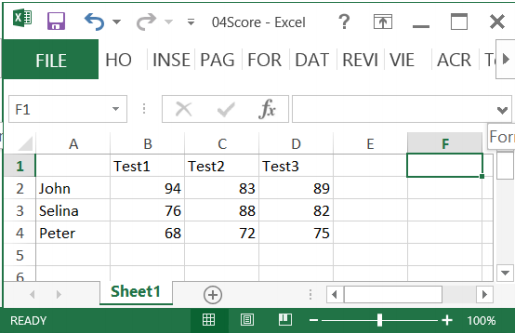
Score = xlsread('04Score.xlsx')
Score = xlsread('04Score.xlsx', 'B2:D4')
[Score Header] = xlsread('04Score.xlsx')

Syntax for writing Excel: xlswrite(filename,A,sheet,xlRange)

M = mean(Score);
xlswrite('04Score.xlsx', M, 1, 'E2:E4');
xlswrite('04Score.xlsx', {'Mean'}, 1, 'E1');

Basic drawing

Drawing and decoration of drawing lines

Use the plot() function to draw lines

In MATLAB, the plot() function is used to draw the plot line, and its syntax is:

plot(x,y,LineSpec)

LineSpec: line setting of drawing line. Three setting characters of specified line type, mark symbol and color form a string. The setting characters are not distinguished in order For details, please refer to Official documents.

Note: the drawing method of matplotlib in Python is almost the same as here

Decorative drawing line

Use the legend() function to add a legend to the picture

Use the legend (label1,..., labeln) function to add a legend to the picture

x=0:0.5:4*pi;
y=sin(x); h=cos(x); w=1./(1+exp(-x)); g=(1/(2*pi*2)^0.5).*exp((-1.*(x-2*pi).^2)./(2*2^2));
plot(x,y,'bd-' ,x,h,'gp:',x,w,'ro-' ,x,g,'c^-');		% Draw multiple lines
legend('sin(x)','cos(x)','Sigmoid','Gauss function');	% Add legend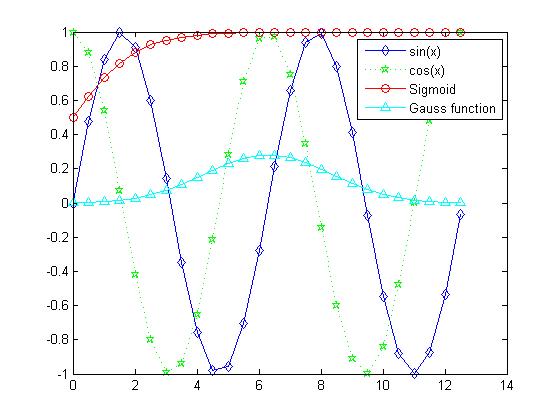

Use title() and * label() to add a title and label to the picture

x = 0:0.1:2*pi; y1 = sin(x); y2 = exp(-x);
plot(x, y1, '--*', x, y2, ':o');
xlabel('t = 0 to 2\pi');
ylabel('values of sin(t) and e^{-x}')
title('Function Plots of sin(t) and e^{-x}');
legend('sin(t)','e^{-x}');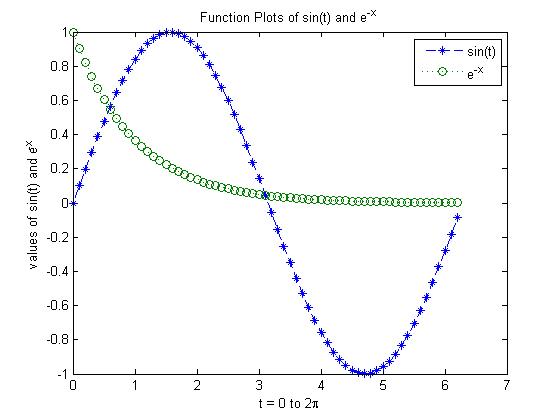

Use text() and annotation() to annotate the picture

x = linspace(0,3); y = x.^2.*sin(x); plot(x,y);
line([2,2],[0,2^2*sin(2)]);
str = '$$ \int_{0}^{2} x^2\sin(x) dx $$';
text(0.25,2.5,str,'Interpreter','latex');
annotation('arrow','X',[0.32,0.5],'Y',[0.6,0.4]);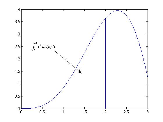 

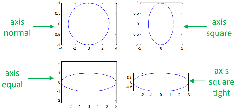
Control axes, borders and grids

The following example demonstrates the effect of the axis command:

t = 0:0.1:2*pi; x = 3*cos(t); y = sin(t);
subplot(2, 2, 1); plot(x, y); axis normal
subplot(2, 2, 2); plot(x, y); axis square
subplot(2, 2, 3); plot(x, y); axis equal
subplot(2, 2, 4); plot(x, y); axis equal tight

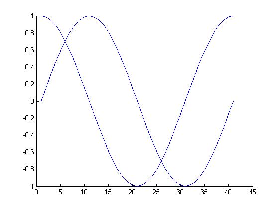
Draw multiple lines

Draw multiple lines on one image

By default, each execution of the plot() function will clear the result of the last drawing, and multiple executions of plot() will only retain the last drawing

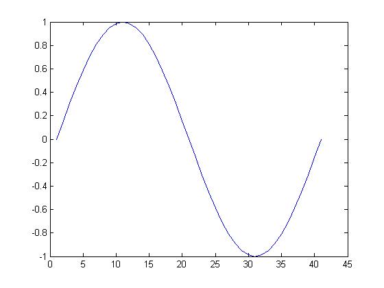
We can use hold on and hold off commands to control the refresh of the drawing area, so that multiple drawing results can be retained in the drawing area at the same time

hold on		% Lift the brush,Start drawing a set of pictures			
plot(cos(0:pi/20:2*pi));
plot(sin(0:pi/20:2*pi));
hold off	% Put down the brush,The group of pictures has been drawn

Draw multiple images in one window

subplot

Operation of drawing objects

In MATLAB, graphics are stored in memory in the form of objects, which can be operated by obtaining their graphic handles

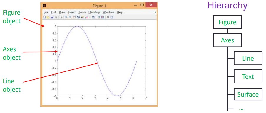
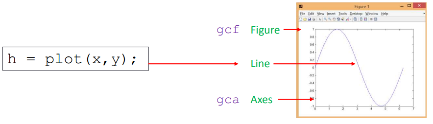
Get graph handle

A graphics handle is essentially a floating point number that uniquely identifies a graphics object The following functions are used to get the graphics handle

All drawing functions also return a handle to the drawing object

Manipulate drawing attributes through drawing handles

Use get() and set() functions to access and modify the properties of graphic objects visit Official documents You can view the properties of all drawing objects

• set(H,Name,Value)
• v = get(h,propertyName)

The following two examples demonstrate the use of graphic handles to manipulate graphic objects:

Change axis properties:

% First picture
set(gca, 'FontSize', 25);

% Second picture
set(gca, 'XTick', 0:pi/2:2*pi);
set(gca, 'XTickLabel', 0:90:360);

% The third picture
set(gca, 'FontName', 'symbol');
set(gca, 'XTickLabel', {'0', 'p/2', 'p', '3p/2', '2p'});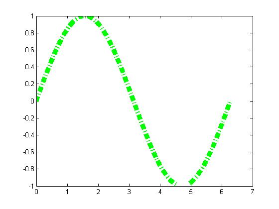

Change Linetype

h = plot(x,y); 
set(h, 'LineStyle','-.', ...
	'LineWidth', 7.0, ...
	'Color', 'g');

Save drawing to file

Use the saveas(fig,filename) command to save graphic objects to a file, where fig is the graphic handle and filname is the file name

saveas(gcf, 'myfigure.png')

Draw advanced charts

Two dimensional chart

Line chart

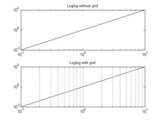
Logarithmic coordinate system line

The following example demonstrates a logarithmic coordinate system line:

x = logspace(-1,1,100); y = x.^2;

subplot(2,2,1);
plot(x,y);
title('Plot');

subplot(2,2,2);
semilogx(x,y);
title('Semilogx');

subplot(2,2,3);
semilogy(x,y);
title('Semilogy');

subplot(2,2,4);
loglog(x, y);
title('Loglog');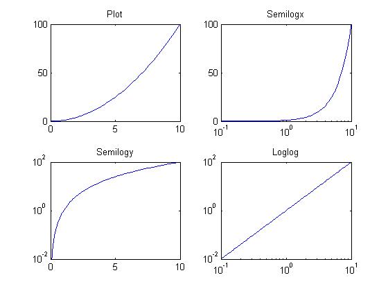 

Logarithmic coordinate system can be added with grid to distinguish linear coordinate system from logarithmic coordinate system

set(gca, 'XGrid','on');

Double y-axis line

The return value of plotyy() is an array [ax,hlines1,hlines2], where:

• ax is a vector that holds handles to objects in two coordinate systems
• hlines1 and hlines2 are handles to two lines respectively

x = 0:0.01:20;
y1 = 200*exp(-0.05*x).*sin(x);
y2 = 0.8*exp(-0.5*x).*sin(10*x);
[AX,H1,H2] = plotyy(x,y1,x,y2);
set(get(AX(1),'Ylabel'),'String','Left Y-axis')
set(get(AX(2),'Ylabel'),'String','Right Y-axis')
title('Labeling plotyy');
set(H1,'LineStyle','--'); set(H2,'LineStyle',':');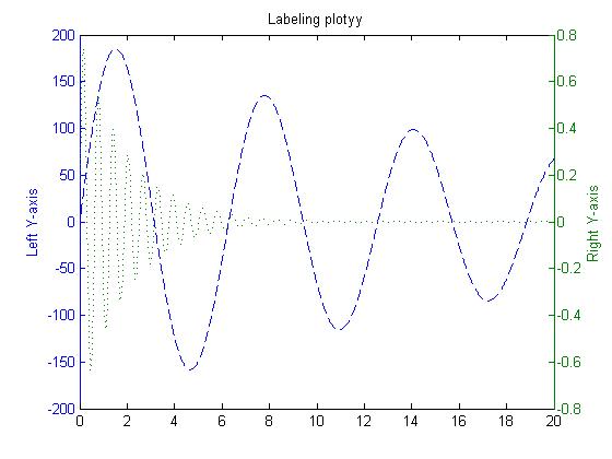

Statistical chart

histogram

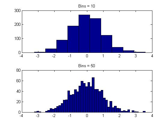
Histogram

Use bar() and bar3() functions to draw two-dimensional and three-dimensional histograms respectively

x = [1 2 5 4 8]; y = [x;1:5];
subplot(1,3,1); bar(x); title('A bargraph of vector x');
subplot(1,3,2); bar(y); title('A bargraph of vector y');
subplot(1,3,3); bar3(y); title('A 3D bargraph');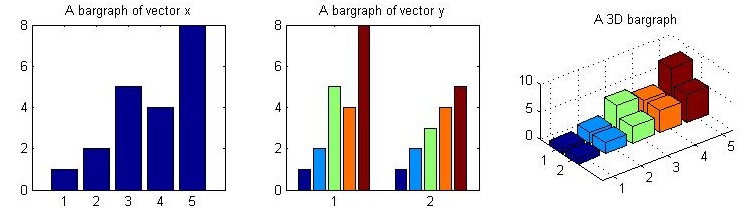

hist is mainly used to view the frequency distribution of variables, while bar is mainly used to view the statistical results of discrete quantities

Using the barh() function, you can draw a histogram arranged vertically

x = [1 2 5 4 8];
y = [x;1:5];
barh(y);
title('Horizontal');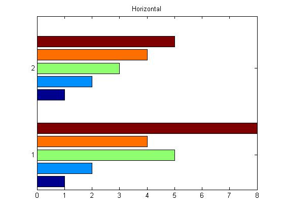

Passing the 'stack' parameter to bar() allows the histogram to be drawn in the form of a stack

x = [1 2 5 4 8];
y = [x;1:5];
bar(y,'stacked');
title('Stacked');

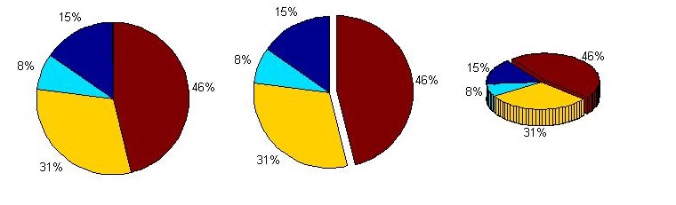
Pie chart

pie() and pie3() can be used to draw 2D and 3D pie charts A bool vector is passed in to indicate whether each sector is offset

a = [10 5 20 30];
subplot(1,3,1); pie(a);
subplot(1,3,2); pie(a, [0,0,0,1]);
subplot(1,3,3); pie3(a, [0,0,0,1]);

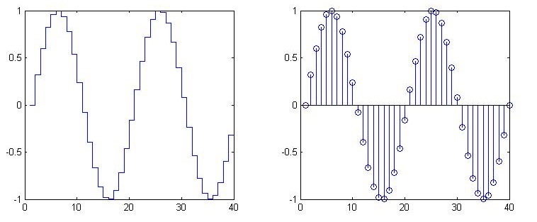
Ladder and needle charts: drawing discrete digital sequences

The stairs() and stem() functions are used to draw a ladder graph and a needle graph, respectively, to represent discrete digital sequences

x = linspace(0, 4*pi, 40); y = sin(x);
subplot(1,2,1); stairs(y);
subplot(1,2,2); stem(y);

Three dimensional chart

Convert 2D to 3D

In MATLAB, all graphs are three-dimensional graphs, and two-dimensional graphs are just a projection of three-dimensional graphs Click the Rotate 3D button in the graphics window to drag and drop the mouse to view the 3D view of the graphics

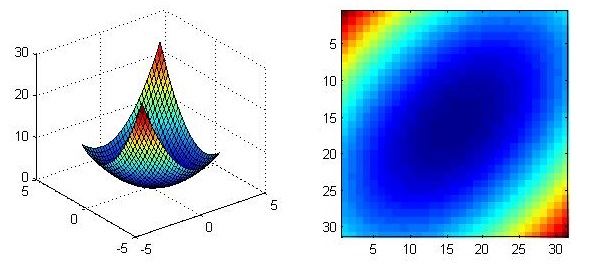
Convert 3D to 2D

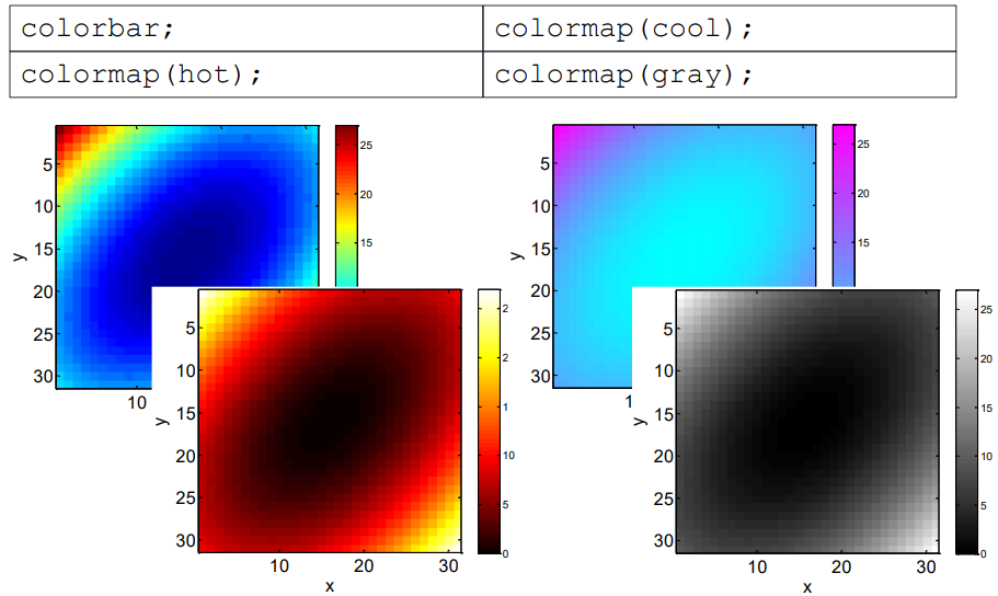
Use the imagesc() function to convert a three-dimensional view into a two-dimensional top view, and indicate the height by the color of the point

[x, y] = meshgrid(-3:.2:3,-3:.2:3); z = x.^2 + x.*y + y.^2; 

subplot(1, 2, 1)
surf(x, y, z); 

subplot(1, 2, 2)
imagesc(z);

Use the colorbar command to add the legend of the corresponding relationship between color and height on the generated two-dimensional map, and use the colormap command to change the color scheme For details, please refer to Official documents

Drawing of three-dimensional drawing

Preparation before drawing 3D drawing

• Using meshgrid() to generate 2D mesh

The meshgrid() function expands the two input vectors by corresponding rows and columns to obtain two augmented matrices. The binary function can be applied to the matrix

x = -2:1:2;
y = -2:1:2;
[X,Y] = meshgrid(x,y)
Z = X.^2 + Y.^2

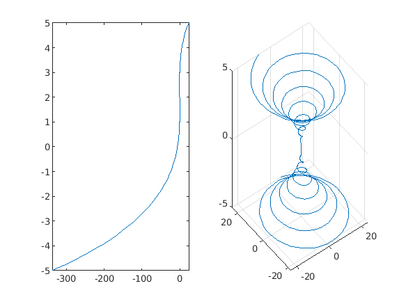
Draw 3D lines

Use the plot3() function to draw a three-dimensional surface. The input should be three vectors

x=0:0.1:3*pi; z1=sin(x); z2=sin(2.*x); z3=sin(3.*x);
y1=zeros(size(x)); y3=ones(size(x)); y2=y3./2;
plot3(x,y1,z1,'r',x,y2,z2,'b',x,y3,z3,'g'); grid on;
xlabel('x-axis'); ylabel('y-axis'); zlabel('z-axis');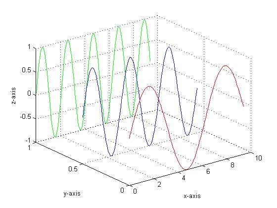

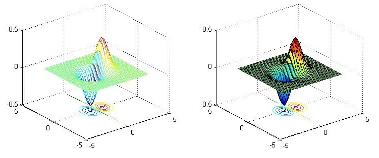
Draw 3D faces

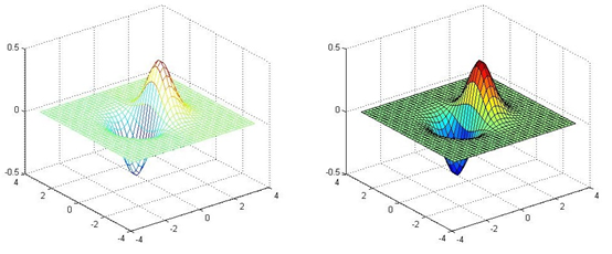
mesh() and surf() commands can be used to draw 3D faces. The former does not fill the mesh, while the latter does

x = -3.5:0.2:3.5; y = -3.5:0.2:3.5;
[X,Y] = meshgrid(x,y);
Z = X.*exp(-X.^2-Y.^2);
subplot(1,2,1); mesh(X,Y,Z);
subplot(1,2,2); surf(X,Y,Z);

Draw contours of 3D graphics

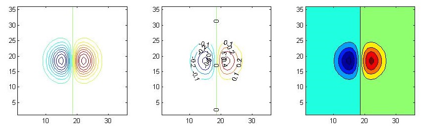
contour() and contour() functions can be used to draw contour lines of 3D graphics. The former does not fill the mesh, while the latter does

The details of the image can be changed by passing parameters or manipulating the graphics handle to the contour() function:

x = -3.5:0.2:3.5; y = -3.5:0.2:3.5;
[X,Y] = meshgrid(x,y); Z = X.*exp(-X.^2-Y.^2);

subplot(1,3,1); contour(Z,[-.45:.05:.45]); axis square;
subplot(1,3,2); [C,h] = contour(Z); clabel(C,h); axis square;
subplot(1,3,3); contourf(Z); axis square;

Using meshc() and surfc() functions, you can draw the contour lines of 3D graphics

x = -3.5:0.2:3.5; y = -3.5:0.2:3.5;
[X,Y] = meshgrid(x,y); Z = X.*exp(-X.^2-Y.^2);

subplot(1,2,1); meshc(X,Y,Z);
subplot(1,2,2); surfc(X,Y,Z);

Draw 3D volume

Use the patch() function to draw a three - dimensional volume

v = [0 0 0; 1 0 0 ; 1 1 0; 0 1 0; 0.25 0.25 1; 0.75 0.25 1; 0.75 0.75 1; 0.25 0.75 1];
f = [1 2 3 4; 5 6 7 8; 1 2 6 5; 2 3 7 6; 3 4 8 7; 4 1 5 8];

subplot(1,2,1); 
patch('Vertices', v, 'Faces', f, 'FaceVertexCData', hsv(6), 'FaceColor', 'flat');
view(3); axis square tight; grid on;

subplot(1,2,2); 
patch('Vertices', v, 'Faces', f, 'FaceVertexCData', hsv(8), 'FaceColor','interp');
view(3); axis square tight; grid on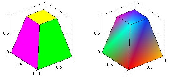

Perspective and lighting of three-dimensional drawings

Adjust Perspective

The view() function can be used to adjust the viewing angle. The view() function accepts two floating-point parameters, representing two azimuth azimuth and elevation

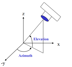
sphere(50); shading flat;
material shiny;
axis vis3d off;
view(-45,20);

Symbolic operation

Create symbolic variable

Create symbolic numbers

Use the sym function to create symbolic numbers Using symbolic numbers can accurately save irrational numbers without error

sym(1/3)	% Get 1/3
1/3			% Get 0.3333

Saving irrational numbers as symbolic numbers can avoid the error of converting them to floating-point numbers:

sin(sym(pi))	% Get 0
sin(pi)			% Get 1.2246e-16

Create symbolic variable

sym and syms can be used to create symbolic variables. The difference is:

sym can only create one symbolic variable at a time, while syms can create multiple symbolic variables at a time

syms a		% sym The command can only create one symbolic variable
syms b c d	% syms Command can create multiple symbolic variables

If the specified symbolic variable already exists, sym will not keep its original value, but syms will clear its value

syms x y
f = x+y;	% Implicitly create symbolic variables f
sym f		% Do not empty variables f Original value,Namely f = x + y

syms x y
f = x+y;	% Implicitly create symbolic variables f
syms f		% Empty variable f Original value,Namely f = f

Using sym, you can create a symbolic variable matrix

A = sym('a', [2 5])	% Create a 2*5 Symbolic variable matrix
whos

The output is as follows:

A =
[ a1_1, a1_2, a1_3, a1_4, a1_5]
[ a2_1, a2_2, a2_3, a2_4, a2_5]
 
 
  Name      Size            Bytes  Class    Attributes
  A         2x5               112  sym      

Using sym and syms together, you can quickly create a series of variables with subscripts

clear all
syms(sym('a', [1 5]))
whos

The output is as follows:

Name      Size            Bytes  Class    Attributes
a1        1x1                 8  sym                
a2        1x1                 8  sym                
a3        1x1                 8  sym                
a4        1x1                 8  sym                
a5        1x1                 8  sym                

Symbolic operation

Simplification and substitution of symbolic expressions

Simplification of symbolic expressions

Use the simplify() function to simplify symbolic expressions

syms x a b c

simplify(sin(x)^2 + cos(x)^2);		% Get 1
simplify(exp(c*log(sqrt(a+b))));	% obtain (a + b)^(c/2)

The standard of expression simplification is uncertain. The following three functions simplify expressions according to different standards:

The expand() function expands the expression

syms x

f = (x ^2- 1)*(x^4 + x^3 + x^2 + x + 1)*(x^4 - x^3 + x^2 - x + 1);
expand(f);		% obtain x^10 - 1

The factor() function can decompose a factor

syms x

g = x^3 + 6*x^2 + 11*x + 6;
factor(g);		% obtain (x + 3)*(x + 2)*(x + 1)

The horner() function can change polynomials into nested forms

syms x

h = x^5 + x^4 + x^3 + x^2 + x;
horner(h);		% obtain x*(x*(x*(x*(x + 1) + 1) + 1) + 1)

Substitution of symbolic expressions

Use the sub(expr, old, new) function to replace old in the symbolic expression expr with new

syms x y

f = x^2*y + 5*x*sqrt(y);
subs(f, x, 3);	% Get 9*y + 15*y^(1/2)

Find the analytical solution of the equation

Using solve(eqn,var) and solve(eqns,vars), the analytical solution of the equation can be obtained

Univariate solution of equation

Define an equation with = = and call the solve function to solve it (if the value to the right of the = = symbol is not specified, the default value to the right of the equation is 0.)

syms x

eqn = x^3 - 6*x^2 == 6 - 11*x;
solve(eqn);		% obtain [1 2 3]

Solving multivariable equations

For multivariable equations, we need to specify which variable to solve

syms x y

eqn = [6*x^2 - 6*x^2*y + x*y^2 - x*y + y^3 - y^2 == 0];
solve(eqn, y);	% obtain [1, 2*x, -3*x]

Solving equations

The equations can be solved by passing the equations into the solve() function

syms u v

eqns = [2*u + v == 0, u - v == 1];
S = solve(eqns,[u v]);	

The solution of the equation can be indexed by variable name and can be substituted into other expressions

S.u;				% Get 1/3
S.v;				% obtain -2/3
subs(3*v + u, S);	% obtain -3/5

Symbolic calculus

Find the limit

Use the limit(expr, var, a) function to find the limit of the symbolic expression expr when the variable var approaches A. add the parameter 'left' or 'right' to specify the left limit or right limit

syms x;
expr = 1/x;

limit(expr,x,0);			% obtain NaN
limit(expr,x,0,'left');		% obtain-Inf
limit(expr,x,0,'right');	% obtain Inf

differential

Using diff(expr, var, n) function, the n-order differential of symbolic expression expr to variable var can be obtained

syms a b c x;
expr = a*x^2 + b*x + c;

diff(expr, a);		% obtain x^2
diff(expr, b);		% obtain x
diff(expr, x);		% obtain b + 2*a*x
diff(expr, x, 2);	% Get 2*a

integral

Using the int(expr, var) function, the indefinite integral of the symbolic expression expr to the variable var can be obtained Use the int(expr, var, [a, b]) function to specify the upper and lower limits for definite integral. A and B can be symbolic expressions

syms x a b
expr = -2*x/(1+x^2)^2;

int(expr, x);			% Get 1/(x^2 + 1)
int(expr, x, [1, 2]);	% obtain -0.3
int(expr, x, [1, Inf]);	% obtain -0.5
int(expr, x, [a, b]);	% Get 1/(b^2 + 1) - 1/(a^2 + 1)

For some functions, MATLAB can't find their integral. At this time, MATLAB will return an unresolved integral form

syms x
int(sin(sinh(x)));	% An integral without solution,MATLAB return int(sin(sinh(x)),

Summation of series

Use symsum (expr, K, [a, b]) to calculate the sum of index k of series expr from a to B

syms k x

symsum(k^2, k)			% obtain k^3/3 - k^2/2 + k/6
symsum(k^2, k, [0 10])	% Get 385
symsum(x^k/factorial(k),k,1,Inf)	% obtain exp(x) - 1

Taylor expansion

Use taylor(expr,var,a) to calculate the Taylor series of the expression expr at var=a

syms x

taylor(exp(x))	% obtain x^5/120 + x^4/24 + x^3/6 + x^2/2 + x + 1
taylor(sin(x))	% obtain x^5/120 - x^3/6 + x
taylor(cos(x))	% obtain x^4/24 - x^2/2 + 1

Draw image

You can draw images for symbolic expressions. The common drawing functions are as follows:

The following example shows the drawing of two-dimensional and three-dimensional line images

subplot(1, 2, 1)
syms x
f = x^3 - 6*x^2 + 11*x - 6;
fplot(f, x)

subplot(1, 2, 2)
syms t
fplot3(t^2*sin(10*t), t^2*cos(10*t), t)

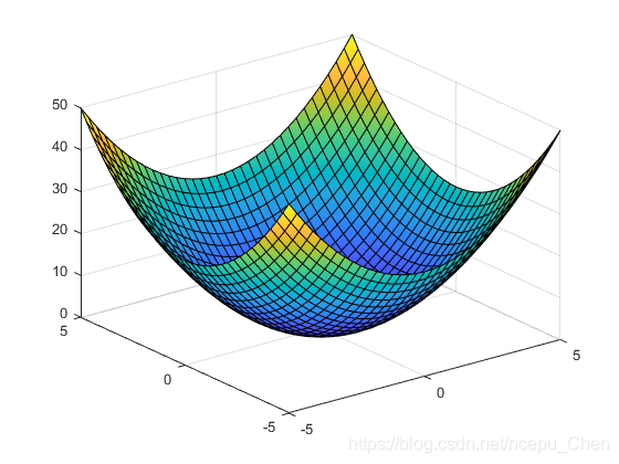
The following example demonstrates the rendering of 3D faces

syms x y
fsurf(x^2 + y^2)

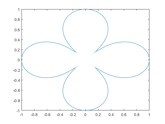
The following example demonstrates the drawing of implicit function relation image

syms x y
eqn = (x^2 + y^2)^4 == (x^2 - y^2)^2;
fimplicit(eqn, [-1 1])

numerical calculation

Numerical operation of polynomials

Polynomial representation using MATLAB

Using vectors to represent polynomials

In MATLAB, polynomials can be represented by vectors. The elements in the vector are the coefficients of polynomials (descending order): the first is the coefficient of the highest order term of polynomials, and the last is the constant term

For example, polynomial: f(x) = x^3 - 2x - 5f(x)=x3−2x−5

It can be represented by vector p = [1 0 -2 -5]

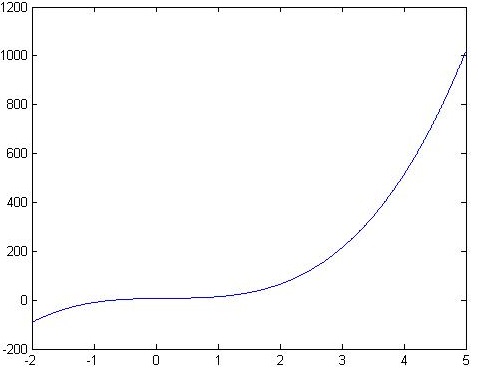
Polynomial evaluation: polyval()

polyval(p, x) can be used to calculate the value of polynomial p at each point of X

a = [9,-5,3,7]; x = -2:0.01:5;
f = polyval(a,x);
plot(x,f);

Multiplication of Polynomials: conv()

Using conv(p1, p2) function, two vectors p1 and p2 can be convoluted and multiplied to calculate the multiplication of polynomials

For example, polynomial: f(x) = (x^2+1) (2x+7)f(x)=(x2+1)(2x+7)

The expanded polynomial can be obtained by using the conv() function:

p = conv([1 0 1], [2 7])

Get p = [2 7 2 7]

Numerical operation of polynomials

Factorization of Polynomials: roots()

The roots(p) function can be used to factorize the polynomial p, that is, to find the root of the expression value of 0

p = roots([1 -3.5 2.75 2.125 -3.875 1.25])

Get p = [2 -1, 1+0.5i, 1-0.5i, 0.5], representing x^5 -3.5 x^4 +2.75 x^3 + 2.125 x^2 + -3.875 x+1.25 = (x-2)(x+1)(x-1-0.5i)(x-1+0.5i)(x-0.5)x5 − 3.5x4+2.75x3+2.125x2 + − 3.875x+1.25=(x − 2)(x+1)(x − 1 − 0.5i)(x − 1+0.5i)(x − 0.5)

Differential of Polynomials: polyder()

The derivative of polynomial can be calculated by using polyder(p) function

For example, take the derivative of the following polynomial: f(x) = 5x^4 - 2x^2 + 1f(x)=5x4−2x2+1

p = polyder([5 0 -2 0 1]);

Get P = [200 - 40], which means that the derivative f '(x) = 20 x^3 - 4xf' (x)=20x3 − 4x

Integral of polynomial: polynomial ()

The polynomial (p, k) function can be used to calculate the integral of polynomial p, and the constant term of the integral result is set to k

For example, take the derivative of the following polynomial: f(x) = 5x^4 - 2x^2 + 1f(x)=5x4−2x2+1

p = polyint([5 0 -2 0 1], 3)

Get p = [1 0 -0.6667 0 1 3], which means the calculated integral \ int f(x) dx = x^5 -0.6667x^3 + x + 3 ∫ f(x)dx=x5 − 0.6667x3+x+3

Numerical operation of nonlinear expression

Root finding of equation (system) (fsolve)

Use fsolve(fun, x0) to find the root of nonlinear equations. Fun is the function handle of the equation to be solved, and x0 is the initial value

Find the solution of equation 1.2x+x\sin(x)+0.3=01.2x+xsin(x)+0.3=0 near x=0x=0

f2 = @(x) (1.2*x+x*sin(x)+0.3);
fsolve(f2,0)	% obtain -0.3500

Solving equations \begin{aligned} \left\{ \begin{aligned} e^{-e^{-(x_1+x_2)}} - x_2(1+x_1^2) = 0 \\ x_1 \cos x_2 + x_2 \sin x_1 - \frac{1}{2} = 0 \end{aligned} \right. \end{aligned}⎩⎪⎨⎪⎧​e−e−(x1​+x2​)−x2​(1+x12​)=0x1​cosx2​+x2​sinx1​−21​=0​​

Set the initial value as [0, 0] [0,0]

fun = @(x) [exp(-exp(-(x(1)+x(2))))-x(2)*(1+x(1)^2)...
    x(1)*cos(x(2)) + x(2)*sin(x(1)) - 0.5]
x0 = [0,0];
x = fsolve(fun,x0)	% obtain[0.3532 0.6061]

Numerical differentiation

Difference: diff()

Use diff(X, n) to calculate the n-order difference of vector X, and N defaults to 1

x = [1 2 5 2 1];
diff(x);	% obtain [1 3 -3 -1]
diff(x,1);	% obtain [1 3 -3 -1]
diff(x,2);	% obtain [2 -6 2]

Derivative: diff (y)/ diff(x)

Use the definition of derivative

You can calculate the approximate derivative of a function at a certain point

The following program calculates the values of the first and second derivatives of f(x) = x^3f(x)=x3

x = -2:0.005:2; y = x.^3;
m = diff(y)./diff(x);			% Calculate the first derivative
m2 = diff(m)./diff(x(1:end-1));	% Calculate the second derivative

plot(x,y,x(1:end-1),m,x(1:end-2),m2);
xlabel('x'); ylabel('y');
legend('f(x) =x^3','f''(x)','f''''(x)', 4);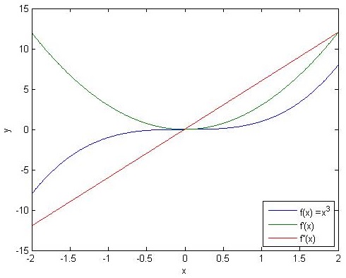

numerical integration

Numerical integration principle

There are three common algorithms used to calculate numerical integration: rectangular method, trapezoidal method and parabola method. They treat the graphics of differential interval as rectangle, trapezoid and parabola respectively to calculate the area

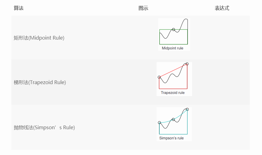
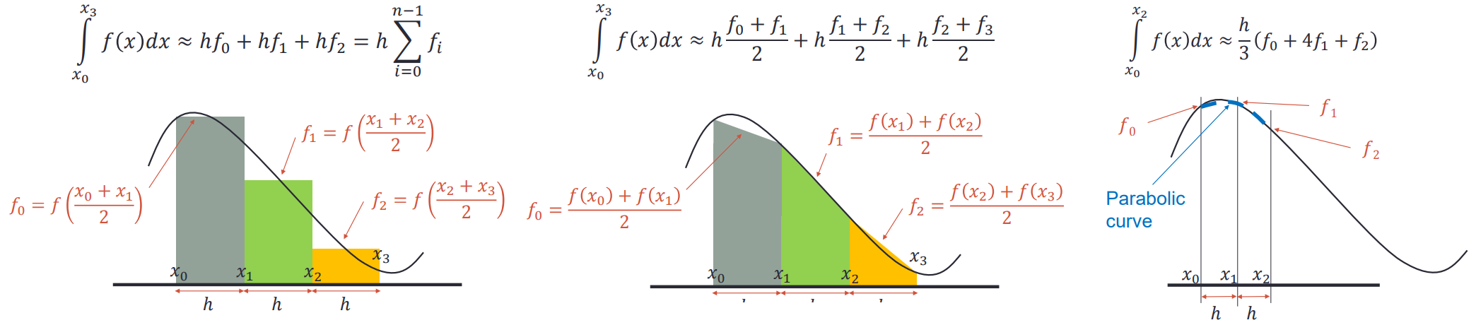
The following three methods are used to calculate the integral of f(x) = 4x^3f(x)=4x3 in the interval (0,2) (0,2)

h = 0.05; x = 0:h:2;


% Use the rectangular method to calculate the approximate integral
midpoint = (x(1:end-1)+x(2:end))./2;
y = 4*midpoint.^3;
s = sum(h*y)			% Get 15.9950

% The trapezoidal method is used to calculate the approximate integral
trapezoid = (y(1:end-1)+y(2:end))/2;
s = h*sum(trapezoid)	% Get 15.2246

% Numerical integration using parabolic method
s = h/3*(y(1)+2*sum(y(3:2:end-2))+4*sum(y(2:2:end))+y(end))	% Get 15.8240

Numerical integration function: integral()

integral(),integral2(),integral3() perform single, double and triple integrals of the function from xmin to xmax respectively

Their first parameter should be a function handle. The following example demonstrates their usage:

Calculate \ int_0^2 \frac{1}{x^3-2x-5}∫02x3−2x−51

f = @(x) 1./(x.^3-2*x-5);
integral(f,0,2)		% obtain -0.4605

Calculate \ int_0^\pi \int_\pi^{2\pi} (y\sin(x) + x \cos(y)) dx dy∫0π∫π2π(ysin(x)+xcos(y))dxdy

f = @(x,y) y.*sin(x)+x.*cos(y);
integral2(f,pi,2*pi,0,pi)	% obtain -9.8696

Calculate \ int_{-1}^1 \int_0^1 \int_0^\pi (y\sin(x) + z \cos(y)) dx dy dz∫−11∫01∫0π(ysin(x)+zcos(y))dxdydz

f = @(x,y,z) y.*sin(x)+z.*cos(y);
integral3(f,0,pi,0,1,-1,1)

Statistics and fitting

Statistics

Descriptive statistics

Descriptive statistics mainly studies the central tendency and Variation of data

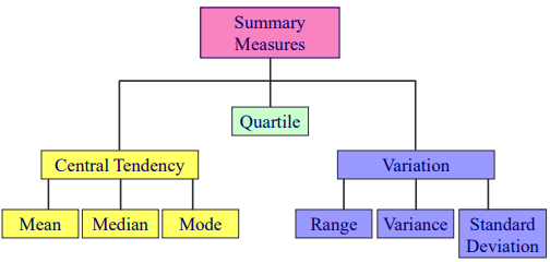
Central trend

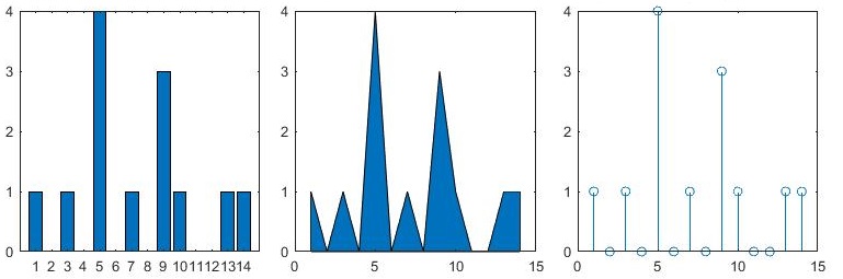
The following functions plot statistical charts:

x = 1:14;
freqy = [1 0 1 0 4 0 1 0 3 1 0 0 1 1];
subplot(1,3,1); bar(x,freqy); xlim([0 15]);
subplot(1,3,2); area(x,freqy); xlim([0 15]);
subplot(1,3,3); stem(x,freqy); xlim([0 15]);

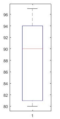
The box chart can highlight the quartile of the data

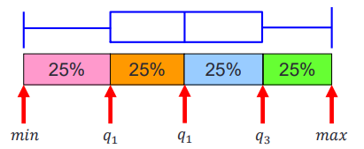
marks = [80 81 81 84 88 92 92 94 96 97];
boxplot(marks) 
% prctile(marks, [25 50 75])	% obtain [81 90 94]

Variation

Degree of dispersion

Skewness

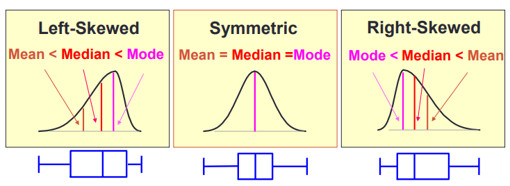
Skewness reflects the degree of symmetry of data

• When the data is biased to the left, its skewness is less than 0
• When the data is completely symmetrical, its skewness is equal to 0
• When the data is biased to the right, its skewness is greater than 0

X = randn([10 3]);		% Structure 10*3 Matrix of
X(X(:,1)<0, 1) = 0; 	% Skew the first column of data to the right
X(X(:,3)>0, 3) = 0;		% Shift the second column of data to the left
boxplot(X, {'Right-skewed', 'Symmetric', 'Left-skewed'});
skewness(X);	% obtain [0.5162 -0.7539 -1.1234]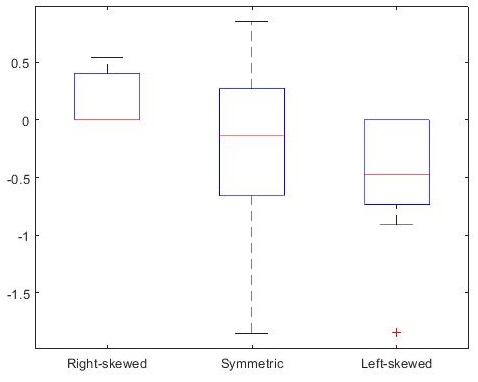

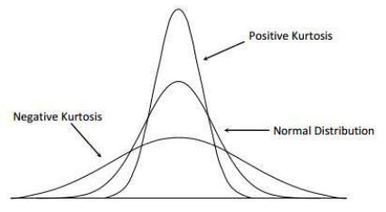
Kurtosis

Kurtosis represents the peak value of probability density distribution curve at the average value Intuitively, kurtosis reflects the sharpness of the peak

Statistical inference

The core of inferential statistics is hypothesis testing The following functions are used for hypothesis testing

load examgrades
x = grades(:,1);
y = grades(:,2);
[h,p] = ttest(x,y);

Executing the above procedure, we get [H P] = [0.9805], which means that we have no reason to refuse the same distribution of x and y under the default significance level (5%)

fitting

Polynomial fitting

Univariate polynomial fitting: polyfit()

The polyfit(x, y, n) function is used to fit the data X and Y polynomially

x = [-1.2 -0.5 0.3 0.9 1.8 2.6 3.0 3.5];
y = [-15.6 -8.5 2.2 4.5 6.6 8.2 8.9 10.0];

for i = 1:3 % Once respectively,secondary,Cubic fitting
    p = polyfit(x, y, i);
    xfit = x(1):0.1:x(end); yfit = polyval(p, xfit);
    subplot(1, 3, i); plot(x, y, 'ro', xfit, yfit);
    legend('Data points', 'Fitted curve', 'Location', 'southeast');
end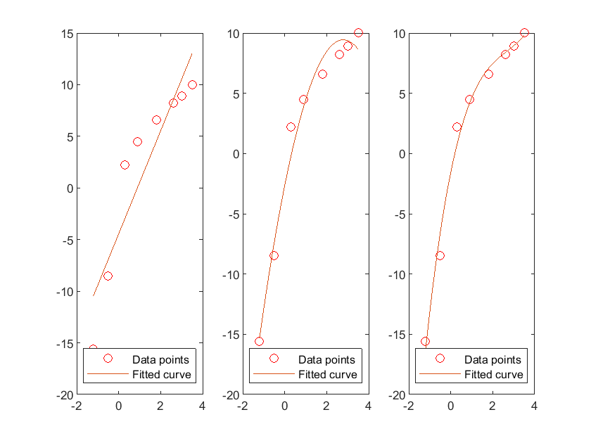

Multivariate linear fitting: regress()

Multiple linear regression is performed on data X and y using the register (y, x) function

load carsmall;
y = MPG; x1 = Weight; x2 = Horsepower;		% Import dataset
X = [ones(length(x1),1) x1 x2];				% Build and expand X matrix
b = regress(y,X);							% Linear regression

% The following is the drawing statement
x1fit = min(x1):100:max(x1); x2fit = min(x2):10:max(x2);
[X1FIT,X2FIT] = meshgrid(x1fit,x2fit);
YFIT = b(1)+b(2)*X1FIT+b(3)*X2FIT;
scatter3(x1,x2,y,'filled'); hold on;
mesh(X1FIT,X2FIT,YFIT); hold off;
xlabel('Weight'); ylabel('Horsepower'); zlabel('MPG'); view(50,10);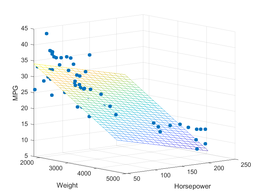

Nonlinear fitting

For nonlinear fitting, curve fitting toolbox is needed Enter cftool() in the command window to open the curve fitting toolbox

interpolation

One dimensional interpolation

The following examples demonstrate linear interpolation using interp1(x, v, xq) and cubic spline interpolation using spline(x, v, xq) The meaning of each parameter is as follows:

• x. V: sample points to be interpolated
• xq: query points. The function returns the interpolation results at these points

% Construction data
x = linspace(0, 2*pi, 40); x_m = x; x_m([11:13, 28:30]) = NaN; 
y_m = sin(x_m);
plot(x_m, y_m, 'ro', 'MarkerFaceColor', 'r'); hold on; 	

% Linear interpolation of data
m_i = ~isnan(x_m);
y_i = interp1(x_m(m_i), y_m(m_i), x);
plot(x,y_i, '-b'); hold on;

% Cubic spline interpolation for data
m_i = ~isnan(x_m);
y_i = spline(x_m(m_i), y_m(m_i), x);
plot(x,y_i, '-g'); 

legend('Original', 'Linear', 'Spline');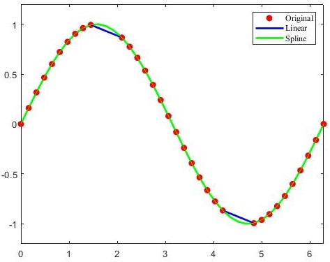

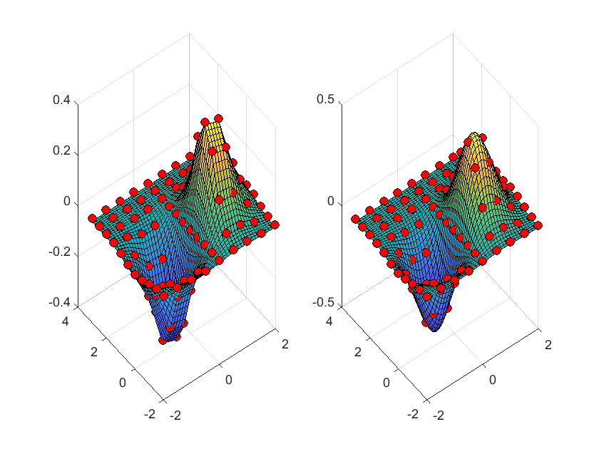
Two dimensional interpolation

interp2() can be used for two-dimensional interpolation, and the interpolation algorithm can be specified by passing a string to its method parameter

% Build sample points
xx = -2:.5:2; yy = -2:.5:3; [x,y] = meshgrid(xx,yy); 
xx_i = -2:.1:2; yy_i = -2:.1:3; [x_i,y_i] = meshgrid(xx_i,yy_i);
z = x.*exp(-x.^2-y.^2);

% linear interpolation
subplot(1, 2, 1); 
z_i = interp2(xx,yy,z,x_i,y_i);
surf(x_i,y_i,z_i); hold on;
plot3(x,y,z+0.01,'ok','MarkerFaceColor','r'); hold on;

% Cubic interpolation
subplot(1, 2, 2); 
z_ic = interp2(xx,yy,z,x_i,y_i, 'spline');
surf(x_i,y_i,z_ic); hold on;
plot3(x,y,z+0.01,'ok','MarkerFaceColor','r'); hold on;