1. MATLAB representation of basic signal
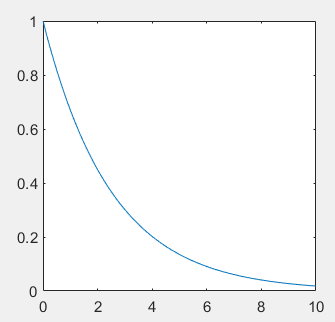
1.1. Exponential signal
%Exponential signal A*exp(a*t)
t = 0:0.1:10;
A = 1;
a = -0.4;
ft = A * exp(a *t );
plot(t,ft)
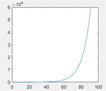
1.2. Exponential series
%Exponential series b^k use.^realization
k = 1:0.1:10;
b = 3;
ft1 =  b.^k;
plot(ft1)
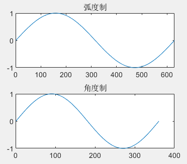
1.3. sine signal
Note that the signal is in radian system (sin) or angle value (sind)
%sinusoidal signal  sin,sind
m = 0:0.01:2*pi;
n = 0:1:360;
ft2 = sin(m);
ft3 = sind(n);
figure(3)
subplot(2,1,1)
plot(ft2)
title('Radian ')
subplot(2,1,2)
plot(ft3)
title('Angle system')
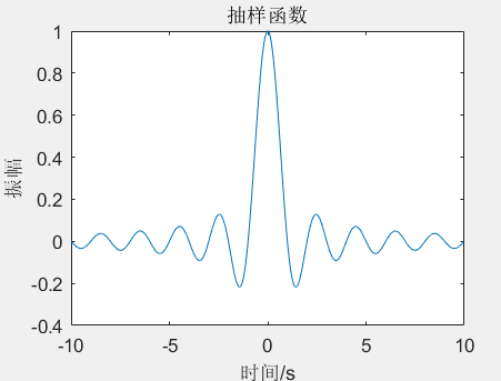
1.4. Sampling function Sa(t)
Sinc(t)
clear all
clc
t = -10:0.01:10;
y = sinc(t);
plot(t,y);
xlabel('time/s');ylabel('amplitude'); title('Sampling function')
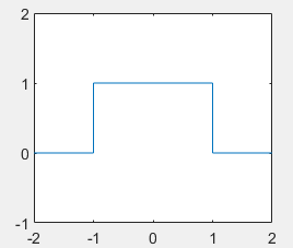
1.5. Rectangular pulse function
rectpuls(t,width)
Generate a rectangular wave signal with amplitude of 1 and width of 2, which is symmetrical about the point t=0. The abscissa range of the function is determined by the vector t, which expands the range of width/2 to the left and right with t=0 as the center, and the default value of width is 1
ylim([yl yr]);: Limit the upper limit value of y-axis, YL: lower limit, yr: upper limit
Axis ([xmin xmax Ymin ymax]): sets the limit range of x-axis and y-axis of the current coordinate axis
%Rectangular pulse
width=2;
t=-2:0.001:3;
ft=rectpuls(t,width);
plot(t,ft)
%ylim([-1 2])
axis([-2,2,-1,2])
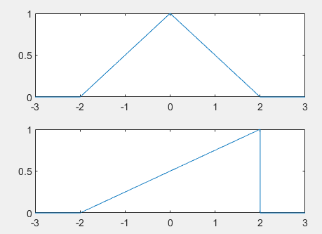
1.6. Triangular wave pulse signal
y=tripuls(T, w, s)
T is an array representing the signal time
w is the width of the triangular wave (the default value is 1)
S is the slope of triangular wave (- 1 < s < 1)
%Triangular wave pulse
t=-3:0.001:3;
ft1=tripuls(t,4,0);
ft2=tripuls(t,4,1);
subplot(2,1,1)
plot(t,ft1)
subplot(2,1,2)
plot(t,ft2)
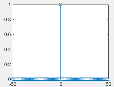
1.7. Unit sampling sequence
Direct generation:
%Unit sampling sequence
k=-50:50;
delta=[zeros(1,50),1,zeros(1,50)];
stem(k,delta)
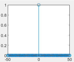
Function generation:
function [f,k]=unitimpuls(k0,k1,k2)
%produce f[k]=delta(k-k0);
%k1<=k<=k2
k=k1:k2;
f=(k-k0)==0;
end
k0 =0;k1=-50;k2=50;
[f,k]=unitimpuls(k0,k1,k2);
stem(k,f)
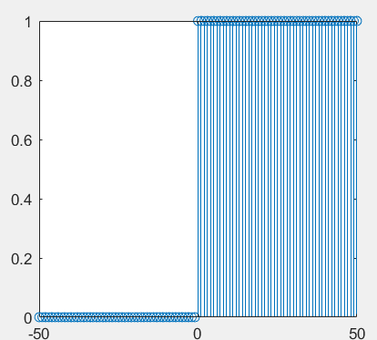
1.8. Unit Step Sequence
Direct generation:
%Unit Step Sequence
k=-50:50;
uk=[zeros(1,50), ones(1,51)];
stem(k,uk)
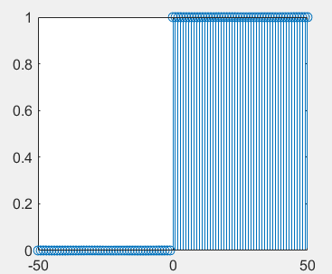
Function generation:
function [f,k] = unitstep(k0,k1,k2)
%produce f[k]=u(k-k0);k1<=k<=k2
k=k1:k2;
f=(k-k0)>=0;
end
k0=0;k1=-50;k2=50;
[f,k]=unitstep(k0,k1,k2);
stem(k,f)
2. MATLAB implementation of basic signal operation
2.1. Scale transformation, inversion and time shift (translation) of signal
Compression: abscissa * n (n > 1 compression, n < 1 expansion)
Flip: abscissa * - 1
Translation: abscissa + - n (left + right -)
%Scale transformation, inversion and time shift (translation) of signal
t=-4:0.001:4;
ft=tripuls(t,4,0.5); % original signal
subplot(2,2,1); plot(t,ft); title('x(t)')
ft1=tripuls(2*t,4,0.5); % compress
subplot(2,2,2); plot(t,ft1); title('x(2t)')
ft2=tripuls(-t,4,0.5); % Flip
subplot(2,2,3); plot(t,ft2); title('x(-t)')
ft3=tripuls(t+1,4,0.5); % translation
subplot(2,2,4); plot(t,ft3); title('x(t+1)')
2.2. Addition and multiplication of signals
Add:+
Multiply:*
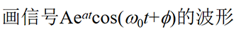
%Draw signal waveform
t=0:0.01:8;
A=1; a=-0.4;
w0=2*pi;phi=0;
ft1=A*exp(a*t).*sin(w0*t+phi);
plot(t,ft1)

2.3. Difference and summation of discrete sequences
Difference: y=diff(f);
y = [f(2)-f(1) f(3)-f(2) ... f(m)-f(m-1)]
Summation: y=sum(f(k1:k2))
y = f(k1)+f(k1+1)+...+f(k2)
2.4. Differentiation and integration of continuous signals
Differential: y=diff(f)/h;
h is the time interval taken for numerical calculation
Definite integral: integral(function_handle,a,b);
function_handle handle of integrand function, a and b definite integral interval
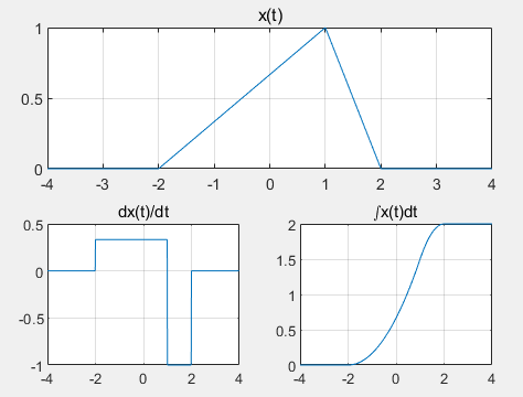
Example: given the triangular wave x(t), draw its differential and integral waveforms
%Known triangular wave x(t),Draw its differential and integral waveforms
% original signal
h=0.01;
t=-4:h:4;
ft=tripuls(t,4,0.5);
subplot(2,1,1);
plot(t,ft);
title('x(t)');
grid on
% differential
y1=diff(ft)*1/h;
subplot(2,2,3)
plot(t(1:length(t)-1),y1);
title('dx(t)/dt')
grid on
% integral
for x=1:length(t)
    y2(x)=integral(@(t) tripuls(t,4,0.5),t(1),t(x));
end
subplot(2,2,4)
plot(t,y2)
title('\intx(t)dt')
grid on
3. Analyze the LTI system with MATLAB
Linear time invariant system (LTI): a system whose parameters do not change with time and meet superposition and time invariance
Analysis method: time domain method or transform domain method, such as Fourier transform, Laplace transform and Z transform
System classification: continuous time system and discrete time system
Description method: constant coefficient differential equation, transfer function or state equation of the system
3.1. Solution of zero state response of continuous time system
y = lsim(sys,x,t)
t: Calculate the sampling point vector of the system response
x: System input signal vector
lsim: for linear time invariant model, any input is given and any output is obtained
sys: LTI system model
- sys = tf(b,a)
- b and a are the coefficient vectors of the right (numerator) and left (denominator) terms of the differential equation, respectively
3.2. Solution of impulse response and step response of continuous system
Impulse response: y = impulse(sys,t)
Step response: y = step(sys,t)
4. Use MATLAB to analyze DTS system
4.1. Solution of unit impulse response of discrete-time system
Unit impulse response: h = impz(b,a,k)
sys: LTI system model
t: Calculate the sampling point vector of the system response
k: Value range of output sequence
b. A: coefficient vectors at the right and left ends of the difference equation
4.2. Calculation of discrete convolution
Discrete convolution: c = conv(a,b)
a. B: vector representation of two sequences to be convoluted
conv function can also be used to calculate the product of two polynomials
5.3/4 case analysis
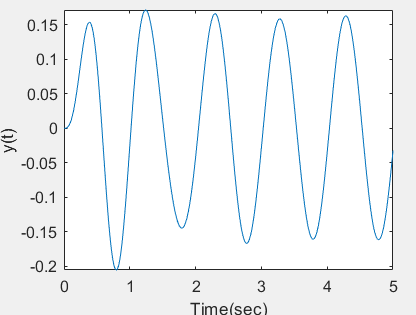
1. Zero state response
Find the zero state response of the system y"(t)+2y '(t)+100y(t)=10x(t), and know that x(t)=sin(2pt) u(t)
%Zero state response of continuous time system
ts=0;te=5;dt=0.01;
sys=tf([10],[1 2 100]);
t=ts:dt:te;
x=sin(2*pi*t);
y=lsim(sys,x,t);
plot(t,y);
xlabel('Time(sec)')
ylabel('y(t)')
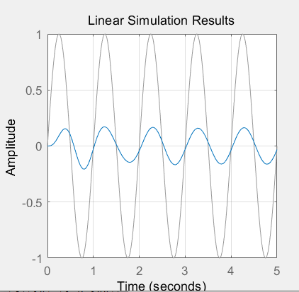
ts=0;te=5;dt=0.01;
sys=tf([10],[1 2 100]);
t=ts:dt:te;
x=sin(2*pi*t);
lsim(sys,x,t);
grid on
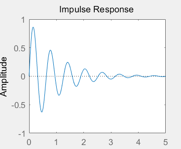
2. Impulse response
Find the impulse response of the system y "(T) + 2Y '(t)+100y(t)=10x(t), and x(t) =d (t)
%Impulse response of continuous time system
ts=0;te=5;dt=0.01;
sys=tf([10],[1 2 100]);
t=ts:dt:te;
y=impulse(sys,t);
plot(t,y);
xlabel('Time(sec)')
ylabel('h(t)')
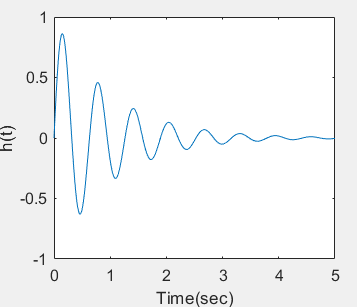
ts=0;te=5;dt=0.01;
sys=tf([10],[1 2 100]);
t=ts:dt:te;
impulse(sys,t)
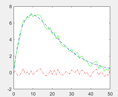
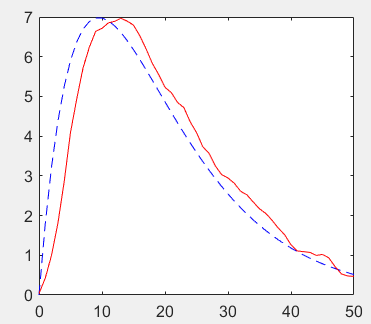
3. Response of moving average system
Analyze the response of the noise interference signal x[k]=s[k]+d[k] through the M-point moving average system
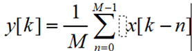
Where s[k]=(2k)0.9^k is the original signal and d[k] is the noise
%Zero state response of discrete-time systems
R =51 ; d = rand(1,R) - 0.5;
k=0:R-1;
s=2*k.*(0.9.^k); x=s+d;
figure(1);
plot(k,d,'r-.',k,s,'b--',k,x,'g-');
M =5; b = ones(M,1)/M; a = 1;
%Filter vector x Data in, vector b by x[k],x[k-1],...Coefficient, vector a by y[k],y[k-1],...Coefficient of
y = filter(b,a,x);
figure(2);
plot(k,s,'b--',k,y,'r-');
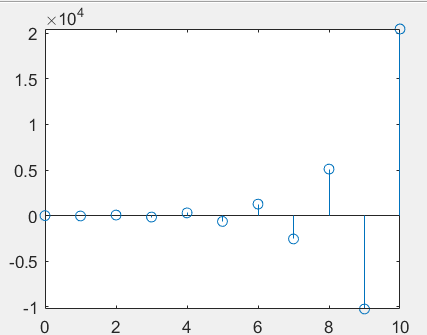
4. Calculate unit impulse response
Find the unit impulse response of the system y[k]+3y[k-1]+2y[k-2]=10x[k]
% Unit impulse response of discrete systems
k=0:10;
a=[1 3 2];
b=[10];
h=impz(b,a,k);
stem(k,h)
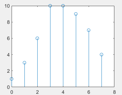
5. Calculate x[k]* y[k] and draw the convolution result
Calculate x[k]* y[k] and draw the convolution result. It is known that x[k]={1,2,3,4; k=0,1,2,3}, y[k]={1,1,1,1,1; k=0,1,2,3,4}
% convolution
x=[1,2,3,4];
y=[1,1,1,1,1];
z=conv(x,y);
N=length(z);
stem(0:N-1,z);
6. Frequency domain analysis of signal using MATLAB
The spectrum Fn is generally complex, and its amplitude frequency characteristics and phase frequency characteristics can be obtained by using abs and angle functions respectively
x = abs(Cn)
y = angle(Cn)
The spectrum Cn of periodic signal is discrete signal, and its spectrum can be drawn by stem
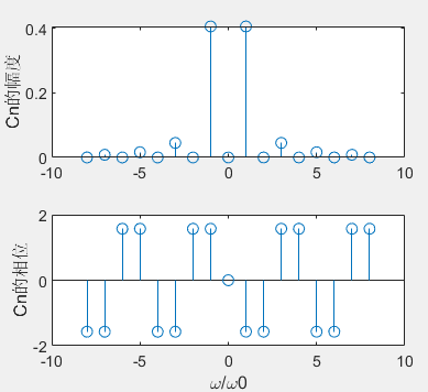
6.1. Draw the spectrum of the periodic triangular wave signal

The spectrum of periodic signal is:

N=8;
%calculation n=-N reach-1 of Fourier coefficient
n1= -N:-1;
c1= -4*j*sin(n1*pi/2)/pi^2./n1.^2;
%calculation n=0 Timely Fourier coefficient
c0=0;
%calculation n=1 reach N of Fourier coefficient
n2=1:N;
c2= -4*j*sin(n2*pi/2)/pi^2./n2.^2;
cn=[c1 c0 c2];
n= -N:N;
subplot(2,1,1);
stem(n,abs(cn));ylabel('Cn Amplitude of');
subplot(2,1,2);
stem(n,angle(cn));
ylabel('Cn Phase of');
xlabel('\omega/\omega0');
6.2. Analysis of aperiodic signal spectrum by numerical integration
y = integral(function_handle,a,b)
Calculate the spectrum of aperiodic signal
function_handle: function handle
a. B: lower and upper limits of definite integral
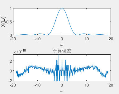
6.2.1. Approximate calculation of the spectrum of triangular wave signal by numerical method

Triangular wave is expressed as:

Theoretical value of triangular wave signal spectrum: X(jw)= Sa^2(w / 2)
sf = @(t,w)(t>=-1 & t<=1).*(1-abs(t)).*exp(-j*w*t);
% Fourier transform formula of triangular pulse signal
w=linspace(-6*pi,6*pi,512);
N=length(w);X=zeros(1,N);
% Numerical integration calculation spectrum
for k=1:N
  X(k)=integral(@(t) sf(t,w(k)),-1,1);
end
subplot(2,1,1);
plot(w,real(X));title('')
xlabel('\omega');ylabel('X(j\omega)');
subplot(2,1,2);
plot(w,real(X)-sinc(w/2/pi).^2);
xlabel('\omega');title('calculation error');
7. Use MATLAB to analyze the frequency domain of the system
7.1. Calculation of frequency response of continuous system
H = freqs(b,a,w)
b: Molecular polynomial coefficient
a: Denominator polynomial coefficient
w: Sampling points of H(jw) to be calculated (the array w needs to contain at least two sampling points of W)
abs: amplitude frequency characteristic
angle: phase frequency characteristic
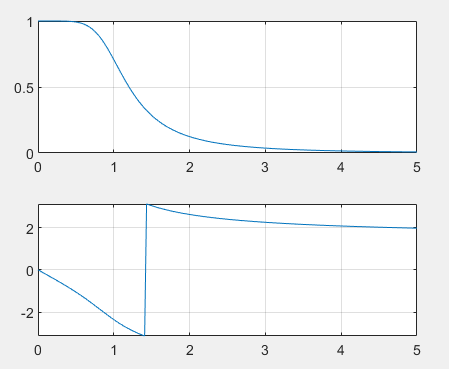
Example: the system function of the third-order normalized Butterworth low-pass filter is

Draw | H(jw) | and φ (w)
w=linspace(0,5,200);
b=[1];a=[1 2 2 1];
h=freqs(b,a,w);
subplot(2,1,1);
plot(w,abs(h))
grid on
subplot(2,1,2);
plot(w,angle(h))
grid on
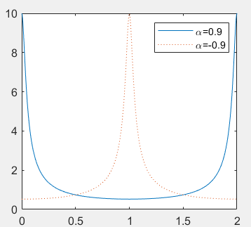
7.2. Calculation of frequency response of discrete system
h = freqz(b,a,w)
b: Molecular polynomial coefficient
a: Denominator polynomial coefficient
w: Sampling points of H(jw) to be calculated (the array w needs to contain at least two sampling points of W)
abs: amplitude frequency characteristic
angle: phase frequency characteristic

b = 1;
a1 = [1 -0.9];
a2 = [1 0.9];
w = linspace(0,2*pi,512);
h1 = freqz(b,a1,w);
h2 = freqz(b,a2,w);
plot(w/pi,abs(h1),w/pi,abs(h2),':')
legend('\alpha=0.9','\alpha=-0.9')
8. Complex frequency domain analysis of continuous system using MATLAB
8.1. MATLAB implementation of partial fraction expansion
[r,p,k] = residue(num,den)
num,den: coefficient vectors of X(s) numerator polynomial and denominator polynomial respectively
r: Coefficient of partial fraction
p: Extreme
k: Polynomial coefficient (if it is true fraction, then K is zero)
Example: find the inverse transformation of X(s) by partial fraction expansion method

format rat %Output the result data in the form of scores
num=[1 2];
den=[1 4 3 0];
[r,p]=residue(num,den)
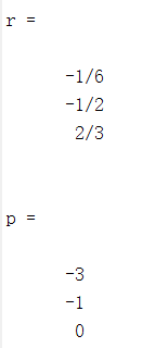
Expanded:

Inverse transformation:

Example: find the inverse transformation of X(s) by partial fraction expansion method

num=[2 3 0 5];
den=conv([1 1],[1 1 2]);
%Convert the form of factor multiplication into the form of polynomial
[r,p,k]=residue(num,den)
magr=abs(r) %seek r Module of
angr=angle(r) %seek r Phase angle of
Operation results:
r =-2.0000 + 1.1339i, -2.0000 - 1.1339i, 3.0000
p =-0.5000 + 1.3229i, -0.5000 - 1.3229i, -1.0000
k =2
magr =2.2291, 2.2991, 3.0000
angr =2.6258, -2.6258, 0
Expanded:

Inverse transformation:

8.2. MATLAB calculation of zero pole and system characteristics of H (s)
r = roots(D)
Calculate the root of polynomial D(s)
[z,p,k] = tf2zp(b,a)
b. a: numerator polynomial coefficient and denominator polynomial coefficient
z: Zero point
p: Extreme
k: Gain constant
pzmap(sys)
Draw the zero pole diagram of the system described by sys
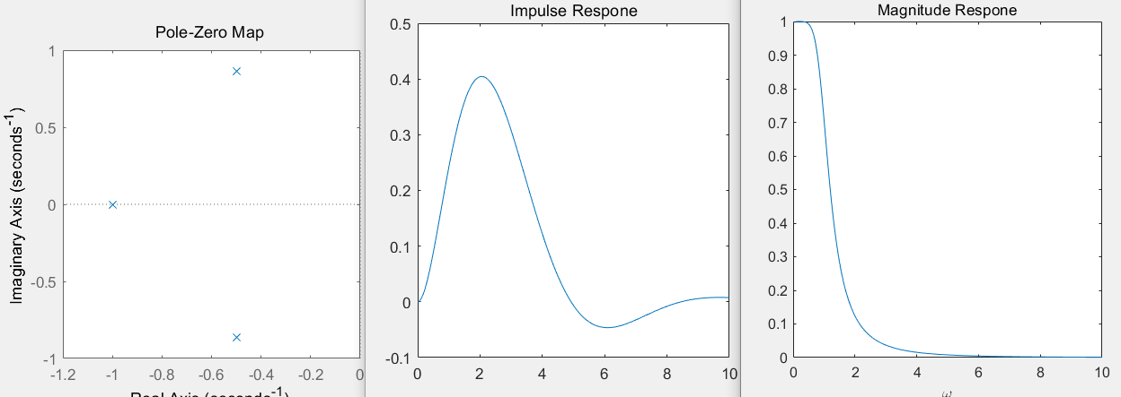
Example: draw the system

The zero pole distribution diagram of, and the unit impulse response h(t) and frequency response H(jw) are obtained
num=[1];den=[1 2 2 1];
sys=tf(num,den);
poles=roots(den)
figure(1);
pzmap(sys);
t=0:0.02:10;
h=impulse(sys,t);
figure(2);
plot(t,h)
title('Impulse Respone')
[H,w]=freqs(num,den);
figure(3);plot(w,abs(H))
xlabel('\omega')
title('Magnitude Respone')
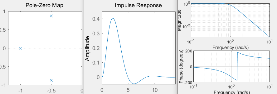
num=[1];den=[1 2 2 1];
sys=tf(num,den);
poles=roots(den)
figure(1);pzmap(sys);
figure(2)
impulse(sys);
figure(3)
freqs(num,den)
9. Use MATLAB to analyze the z-domain of discrete system
9.1. MATLAB implementation of partial fraction expansion
[r,p,k] = residuez(num,den)
num, den: coefficient vectors of numerator polynomials and denominator polynomials
r: Coefficient of partial fraction
p: Extreme
k: Polynomial coefficient, if it is true fraction, then K is zero
Example: expand X(z) with partial fraction

num = [18];
den = [18 3 -4 -1];
[r,p,k] = residuez(num,den)
Operation results
r =0.3600 , 0.2400 , 0.4000
p =0.5000 , -0.3333 , -0.3333
k =[]
Expanded:

8.2. MATLAB calculation of zero pole and system characteristics of H (z)
[z,p,k] = tf2zpk(b,a)
b. a: coefficient vector of numerator polynomial and denominator polynomial
z: Zero point
p: Extreme
k: Gain constant
zplane(b,a)
Draw pole zero distribution diagram
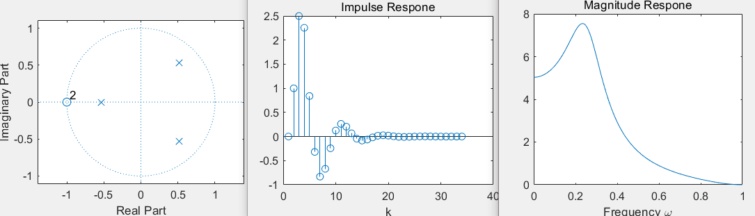
Example: draw the system

The zero pole distribution diagram of, and the unit impulse response h[k] and frequency response H(e^j Ω) are obtained
b =[0 1 2 1];a =[1 -0.5 -0.005 0.3];
figure(1);
zplane(b,a);
num=[0 1 2 1];
den=[1 -0.5 -0.005 0.3];
h=impz(num,den);
figure(2);
stem(h)
xlabel('k')
title('Impulse Respone')
[H,w]=freqz(num,den);
figure(3);
plot(w/pi,abs(H))
xlabel('Frequency \omega')
title('Magnitude Respone')
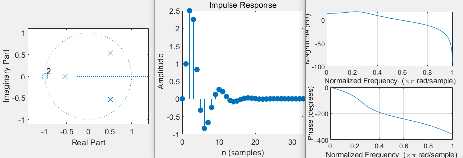
b =[0 1 2 1];a =[1 -0.5 -0.005 0.3];
figure(1);
zplane(b,a);
num=[0 1 2 1];
den=[1 -0.5 -0.005 0.3];
figure(2);
impz(num,den);
figure(3);
freqz(num,den);
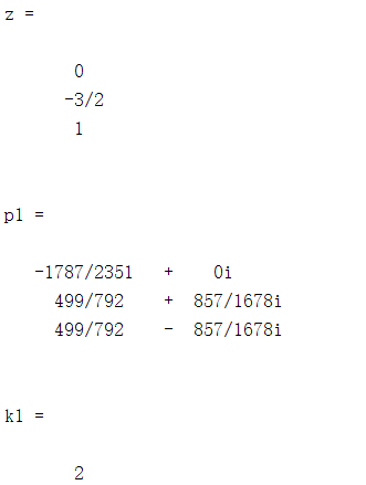
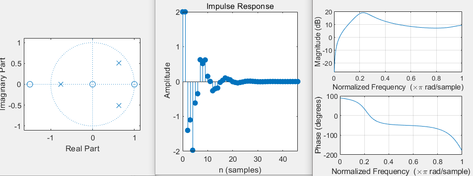
Example: find the system
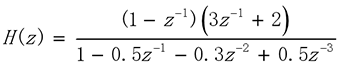
The values of zero and pole, unit impulse response and frequency response
b=conv([1,-1],[2,3]); a=[1 -0.5 -0.3 0.5];
[z,p1,k1]=tf2zpk(b,a)
figure(1)
zplane(b,a);
figure(2)
impz(b,a);
figure(3)
freqz(b,a)