G = graph(s,t,weights) -- use node pair group s,t and weight vector weights
Create weighted undirected graph
G = graph(s,t,weights,nodes) -- use character vector cell array nodes
Specify node name
G = graph(s,t,weights,num) -- use the numerical scalar num to specify the value in the graph
Number of nodes
G = graph(A[,nodes],type) - constructed using only the upper or lower triangular matrix of A
Weighting graph, type can be 'upper' or
'lower'
sparse adjacency matrix to coefficient matrix

Example 1 undirected graph

clc, clear, close all 
E=[1,2;1,3;2,3;3,2;3,5;4,2;4,6;5,2;5,4;6,5] 
s = E(:,1); t = E(:,2); 
nodes =cellstr(strcat('v',int2str([1:6]'))) 
G = digraph(s, t, [], nodes); 
plot(G) 
W1 = adjacency(G) %Coefficient matrix of adjacency matrix 
W2 = incidence(G)%Coefficient matrix of incidence matrix

Clear all: clear all variables, functions, MEX files and strcat in the workspace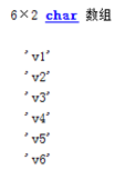
cellstr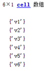
The adjacency matrix represents the relationship between nodes, and the incidence matrix represents the relationship between nodes and edges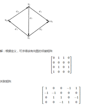

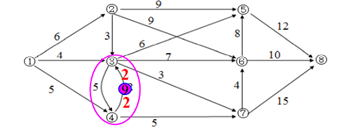
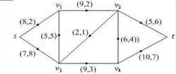
Example 2 shortest path of weighted undirected graph

clc, clear, close all 
E = [1,2,50; 1,4,40; 1,5,25; 1,6,10; 2,3,15; 2,4,20; 2,6,25; 
3,4,10;3,5,20; 4,5,10; 4,6,25; 5,6,55]; 
G = graph(E(:,1), E(:,2), E(:,3)); 
p = plot(G,'EdgeLabel',G.Edges.Weight,'Layout', 'circle');
[path2, d2] = shortestpath(G, 1, 2) %Find the shortest path from 1 to 2
highlight(p,path2,'EdgeColor','r','LineWidth',1.5)%Draw in the picture path2 Route
[path3, d3] = shortestpath(G, 1, 3, 'method','positive') %ditto,'method','positive'Can be omitted
highlight(p,path3,'EdgeColor', 'm','LineWidth',1.5) 

Another example

clc, clear, close all
a(1,2)=2;a(1,3)=8;a(1,4)=1;a(2,3)=6;a(2,5)=1;
a(3,4)=7;a(3,5)=5;a(3,6)=1;a(3,7)=2;a(4,7)=9;
a(5,6)=3;a(5,8)=2;a(5,9)=9;a(6,7)=4;a(6,9)=6;
a(7,9)=3;a(7,10)=1;a(8,9)=7;a(8,11)=9;
a(9,10)=1;a(9,11)=2;a(10,11)=4;
a=a';
[i,j,v]=find(a);
b=sparse(i,j,v,11,11);
[x,y,z]=graphshortestpath(b,1,11,'directed',false)

Where z represents the penultimate node from 1 (set in graphsorestpath, not the default) to the shortest path of each point, for example, z3=6, and the shortest path from 1 to 3 is from 1 to 2 to 5 to 6 and then to 3
It can be seen from the two examples that the shortestpath is used for the generated graph and the graphshortestpath is used for the sparse matrix. The graphmaxflow and maxflow in Example 7 below are the same

Example 3 Dijkstra

clc, clear, a=zeros(6);
a(1,[2,4,5,6])=[50,40,25,10]; 
a(2,[3,4,6])=[15,20,25];
a(3,[4,5])=[10,20]; 
a(4,[5,6])=[10,25];
a(5,6)=55; 
G = graph(a,'upper'); 
d = distances(G,'Method','positive')

Example 4 Prime to find the minimum spanning tree (it seems that it can't be used)

a=zeros(7); 
a(1,2)=50; a(1,3)=60; a(2,4)=65; a(2,5)=40; a(3,4)=52; 
a(3,7)=45; a(4,5)=50; a(4,6)=30;a(4,7)=42; a(5,6)=70; 
a=a+a'; 
a(find(a==0))=inf; 
result=[];p=1;tb=2:length(a); 
while size(result,2)~=length(a)-1 
    temp=a(p,tb); 
    temp=temp(:); 
    d=min(temp); 
     [jb,kb]=find(a(p,tb)==d,1); 
    j=p(jb);k=tb(kb); 
    result=[result,[j;k;d]];p=[p,k];tb(find(tb==k))=[]; 
end 
result

Example 5 Kruskal finds the minimum spanning tree (it seems that it can't be used)

a(1,2)=50; a(1,3)=60; a(2,4)=65; a(2,5)=40;a(3,4)=52;a(3,7)=45; 
a(4,5)=50; a(4,6)=30;a(4,7)=42; a(5,6)=70; 
[i,j,b]=find(a);data=[i';j';b'];index=data(1:2,:); 
loop=length(a)-1;result=[]; 
while length(result)<loop 
     temp=min(data(3,:)); 
     flag=find(data(3,:)==temp);
     flag=flag(1);                   
     v1=index(1,flag);
     v2=index(2,flag);                         
     if v1~=v2 
        result=[result,data(:,flag)];       
     end 
                                             
     index(find(index==v2))=v1;                  
     data(:,flag)=[];index(:,flag)=[];            
end                                               
result 

Example 6 minimum spanning tree function

clc, clear, close all, a=zeros(7); 
a(1,[2 3])=[50,60];a(3,[4,7])=[52,45]; 
a(2,[4 5])=[65 40]; a(4,[5:7])=[50,30,42]; 
a(5,6)=70; 
s=cellstr(strcat('v',int2str([1:7]'))); 
G=graph(a,s,'upper'); 
p=plot(G,'EdgeLabel',G.Edges.Weight) 
T=minspantree(G,'Method','sparse') 
L=sum(T.Edges.Weight), highlight(p,T) 

sum is the weight of the minimum spanning tree, which is often used to connect each point and calculate the minimum weight. Upper indicates that the input matrix is the upper triangle, and vice versa
Another example

clc, clear, xy=load('data4_12.txt'); d=mandist(xy); %seek xy Absolute value distance between two columns of vectors 
s=cellstr(strcat('v',int2str([1:9]'))); %Construct vertex string 
G=graph(d,s); %Structural undirected graph 
T=minspantree(G); %Use default Prim Algorithm for minimum spanning tree 
L=sum(T.Edges.Weight) %Calculate the weight of the minimum spanning tree T.Edges %Displays the edge set of the minimum spanning tree h=plot(G,'Layout','circle','NodeFontSize',12); %Draw an undirected graph 
highlight(h,T,'EdgeColor','r','LineWidth',2) %Thicken the edges of the minimum spanning tree

Example 7 find the maximum flow and label

clc, clear, close all
a = zeros(6); a(1,[2,4])=[8,7]; 
a(2,[3,4])=[9,5]; a(3,[4,6])=[2,5]; 
a(4,5)=9; a(5,[3,6])=[6,10]; 
G = digraph(a);
H=plot(G,'EdgeLabel',G.Edges.Weight); 
[M,F]=maxflow(G,1,6)           
F.Edges, highlight(H,F, 'EdgeColor','r','LineWidth',1.5)

The command graphmaxflow of Matlab Graph Theory toolbox to solve the maximum flow can only solve the problem that the weights are positive and there can be no two arcs between two vertices. If there are two vertices, you can add a virtual vertex. For example, add a virtual vertex 9 between vertex 4 and vertex 3, and add two arcs. Delete the arc with the weight of 2 from vertex 4 to vertex 3. The capacity of both arcs is 2, not 1, because this is the capacity. This one needs the capacity of 2, not the distance.

The minimum cost maximum flow problem requires a maximum flow from the sending point s to the receiving point t, so that the sum of the total transportation cost bf of the flow is the minimum
function [flow,val]=mincostmaxflow(rongliang,cost,flowvalue);
%Minimum cost maximum flow function
%The first parameter: capacity matrix; The second parameter: cost matrix;
%The first two parameters must be disposed of as zero in the non path
%The third parameter: specify the capacity value (can not be written, which means to find the minimum cost and maximum flow)
%The return value flow is the feasible flow matrix, and val is the minimum cost value

Example 8 finding the maximum flow and minimum cost

global M num
c=zeros(6);u=zeros(6);
c(1,2)=2;c(1,4)=8;c(2,3)=2;c(2,4)=5;
c(3,4)=1;c(3,6)=6;c(4,5)=3;c(5,3)=4;c(5,6)=7;
u(1,2)=8;u(1,4)=7;u(2,3)=9;u(2,4)=5;
u(3,4)=2;u(3,6)=5;u(4,5)=9;u(5,3)=6;u(5,6)=10;
num=size(u,1);M=sum(sum(u))*num^2;
[f,val]=mincostmaxflow(u,c)
Two external functions need to be added
firstly

function path=floydpath(w) 
global M num
w=w+((w==0)-eye(num))*M;
p=zeros(num);
for k=1:num
    for i=1:num
        for j=1:num
            if w(i,j)>w(i,k)+w(k,j)
               w(i,j)=w(i,k)+w(k,j);
               p(i,j)=k;
            end
        end
    end
end
if w(1,num)==M
    path=[];
else
    path=zeros(num);
    s=1;
    t=num; m=p(s,t);
    while ~isempty(m)
        if m(1)
            s=[s,m(1)];t=[t,t(1)];t(1)=m(1);
            m(1)=[];
            m=[p(s(1),t(1)),m,p(s(end),t(end))];
        else
            path(s(1),t(1))=1;s(1)=[];m(1)=[];t(1)=[];
        end
   end
end

second

function [flow,val]=mincostmaxflow(rongliang,cost,flowvalue); 
global M 
flow=zeros(size(rongliang));
allflow=sum(flow(1,:)); 
if nargin<3 
    flowvalue=M; 
end
while allflow<flowvalue
    w=(flow<rongliang).*cost-((flow>0).*cost)'; 
    path=floydpath(w); 
    if isempty(path) 
        val=sum(sum(flow.*cost)); 
        return; 
    end 
theta=min(min(path.*(rongliang-flow)+(path.*(rongliang-flow)==0).*M)); 
theta=min([min(path'.*flow+(path'.*flow==0).*M),theta]);
flow=flow+(rongliang>0).*(path-path').*theta; 
allflow=sum(flow(1,:)); 
end 
val=sum(sum(flow.*cost));

For two new functions, click the above run (F9 doesn't seem to work), automatically name them "function name. m", select "add to path", run them separately, and you will be prompted that the input parameters are insufficient, and then run the main file

Common functions

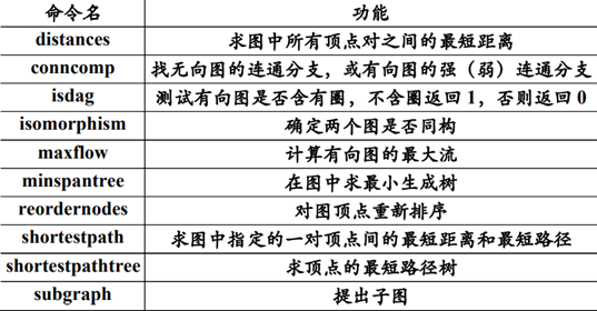
Traveling salesman problem: in graph theory terms, it is to find a Hamilton ian cycle with minimum weight in a weighted complete graph (each pair of different vertices is connected by exactly one edge). This kind of circle is called the optimal circle. At present, the better algorithm is to select two points vi and vj from the obtained circle each time, and compare v(i)v(j)+v(i+1)v(j+1) and v(i)v(i+1)+v(j)v(j+1) for iteration
Example 9 travel agent

clc, clear, close all
global a 
a=zeros(6); 
a(1,2)=56;a(1,3)=35;a(1,4)=21;a(1,5)=51;a(1,6)=60;
a(2,3)=21;a(2,4)=57;a(2,5)=78;a(2,6)=70; a(3,4)=36;
a(3,5)=68;a(3,6)=68; a(4,5)=51;a(4,6)=61;a(5,6)=13;
a=a+a';L=size(a,1); %Returns the number of rows of the matrix, and 2 is the number of columns
c1=[5 1:4 6 ]; %5/1: 4/6
[circle,long]=modifycircle(c1,L); %
c2=[5 6 1:4 ]; %By changing the initial circle, the last vertex of the algorithm is fixed
[circle2,long2]=modifycircle(c2,L);
if long2<long
    long=long2;
    circle=circle2;
end
circle,long
 External function
function [circle,long]=modifycircle(c1,L); 
global a 
flag=1; 
while flag>0 
    flag=0;
    for m=1:L-3 
        for n=m+2:L-1 
            if a(c1(m),c1(n))+a(c1(m+1),c1(n+1))<a(c1(m),c1(m+1))+a(c1(n),c1(n+1)) 
                flag=1; 
                c1(m+1:n)=c1(n:-1:m+1); 
             end 
        end 
    end 
end 
long=a(c1(1),c1(L)); 
for i=1:L-1
    long=long+a(c1(i),c1(i+1)); 
end 
circle=c1;

If the solution of graph theory is not used, linear 0-1 programming can also be used

Example 10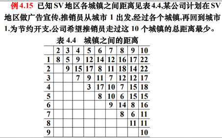

clc, clear
a=readmatrix('data4_15.xlsx');
a(isnan(a))=0; %hold NaN Replace with 0
b=zeros(10); %Adjacency matrix initialization
b([1:end-1],[2:end])=a; %Assignment of triangular elements on adjacency matrix
b=b+b'; %Construct complete adjacency matrix
n=10; 
b([1:n+1:end])=1000000; %Replace diagonal elements with sufficiently large ones
prob=optimproblem; 
x=optimvar('x',n,n,'Type','integer','LowerBound',0,'UpperBound',1);
u=optimvar('u',n,'LowerBound',0) %Sequence number variable
prob.Objective=sum(sum(b.*x));
prob.Constraints.con1=[sum(x,2)==1; sum(x,1)'==1; u(1)==0];con2 = [1<=u(2:end); u(2:end)<=14];
for i=1:n
    for j=2:n
        con2 = [con2; u(i)-u(j)+n*x(i,j)<=n-1];
    end
end
prob.Constraints.con2 = con2;
[sol, fval, flag]=solve(prob)
xx=sol.x; [i,j]=find(xx); 
fprintf('xij=1 The corresponding row and column positions are as follows:\n')
ij=[i'; j']

Where b([1:n+1:end])=1000000; The principle of matrix b is that the elements of matrix b are sorted by column and recorded as b(n). For example, the order of matrix elements of 3 * 3 is