Two Methods of Adding Legends
1. [Recommended use] Add label parameter to plot function, then add plt.legend()
plt.plot(x, x*3.0, label='Fast')
plt.plot(x, x/3.0, label='Slow')
plt.legend()
2. The list of incoming strings in the legend method
plt.plot(x,np.sin(x),x,np.cos(x))
plt.legend(["sin","cos"])
Next is the reading notes of two articles (annotate the places you don't understand)
Chapter 1:
When drawing with python's matplotlib, it is often necessary to add illustrations. If no parameters are set, the default is the best place to add to the inside of the image.
If you need to move the legend to the outside of the image, there are several ways. Here's one.
In the plt.legend() function, several parameters are added: plt.legend(bbox_to_anchor=(num1, num2), loc=num3, borderaxespad=num4). As long as these parameters are added and given a certain value, the legend will be placed outside.
Specific Settings Reference Articles: https://blog.csdn.net/Poul_henry/article/details/82533569
Chapter 2: Link to the original: https://blog.csdn.net/Poul_henry/article/details/88311964
As mentioned last time, when using the following code to save vector maps, the legend on the outside often shows incompleteness:
import numpy as np
import matplotlib.pyplot as plt

fig, ax = plt.subplots()
'''fig,ax = plt.subplots() is equivalent to:
fig = plt.figure()
ax = fig.add_subplot(1,1,1)

fig, ax = plt.subplots(1,3), where parameters 1 and 3 represent the number of rows and columns of subgraphs, respectively. There are 1 x 3 subimages. The function returns an array list of figure images and subgraphs ax.
fig, ax = plt.subplots(1,3,1), and the last parameter 1 represents the first subgraph.
If you want to set the width and height of the subgraph, you can add figsize values to the function
 fig, ax = plt.subplots(1,3,figsize=(15,7)), so there will be one row of three subgraphs of 15x7 size. ''

x1 = np.random.uniform(-10, 10, size=20)
x2 = np.random.uniform(-10, 10, size=20)
# x1, x2 are random arrays with uniform U(-10, 10) distribution

number = []
x11 = []
x12 = []
for i in range(20):
    number.append(i+1)
    x11.append(i+1)
    x12.append(i+1)
'''Last number, x11, x12= [1, 2,..., 20]'''

plt.figure(1)
# plt.figure(1) is a new drawing window named Figure 1

plt.plot(number, x1, 'bo', markersize=20,label='a')  # blue circle with size 20
plt.plot(number, x2, 'ro', ms=10,label='b')  # ms is just an alias for markersize
 '''optional parameter [fmt] is a string that defines the basic attributes of a graph, such as color, marker, linestyle.
The specific form of fmt is'[color] [marker] [line]'. fmt receives a single letter abbreviation for each attribute, such as plot (x, y,'bo-')# blue dot solid line.
So here bo is the blue dot, ro is the red dot'''

lgnd=plt.legend(bbox_to_anchor=(1.05, 1), loc=2, borderaxespad=0,numpoints=1,fontsize=10)
lgnd.legendHandles[0]._legmarker.set_markersize(16)
lgnd.legendHandles[1]._legmarker.set_markersize(10)
 ''bbox_to_anchor: Represents the location of legend, with the former representing left and right, and the latter representing up and down.
 In the binary given bbox_to_anchor, the first value is used to control the left-right movement of legend. The larger the value, the more it moves to the right.
 The second value is used to control the up and down movement of legend. The larger the value, the more upward movement.
 In order to be beautiful, it is necessary to place the legend on the outside of the image, but the distance is not too large. Generally, num1=1.05 is set.
 loc=2 means upper left, in the upper left corner.
 Therefore, when we set bbox_to_anchor=(1.05, 0), that is, legend in the lower right corner of the image, for beauty, we need to place the lower left corner of legend, that is,'lower left'at this point, corresponding to the table's'Location Code' number is 2, that is, num3 is set to 2 or directly set to'upper'; and when we set bbox_to_anchor=(1.05, 1), that is, L upper. When egend is placed in the upper right corner of the image, in order to be beautiful, it is necessary to place the upper left corner of legend, i.e.'upper left', corresponding to the table's'Location Code'number of 3, that is to say, the parameter num3 is set to 3 or directly set to'lower left'.

 borderaxespad represents filling between axes and legend borders. It is measured by font size and distance. The default value is None. But in practice, if this parameter is not added, the effect is certain filling. Equal to 0 indicates alignment.
 numpoints denote the number of points in a line legend'''

plt.show()
fig.savefig('scatter.png',dpi=600)
After being saved as scatter.png, the effect is as follows:
You can see that the legend on the right of the image shows only a small portion on the left.
The reason here is simple. When saving vector graph with savefig() function, it uses a bounding box (bbox, boundary box) to frame the scope. Only the image that falls into the box is saved. If the legend does not fall into the box completely, it can not be saved naturally.
Understand its principle, and then solve the problem is relatively simple.
Here are two solutions:
-
If the image that does not fall into the bbox is completely dropped into the frame by moving it, then the image intercepted by the bbox is complete (the image is moved into the bbox);
-
Change the size of the bbox to include the image completely, especially the legend that often falls outside the bbox (expand the bbox to include the image completely).
Following are two ways to solve this problem based on these two ideas:
- Using the function subplots_adjust()
As can be seen in the official document, the function of subplots_adjust() is to adjust the layout of subgraphs. It contains six parameters, four of which are left, right, bottom and top. The other two parameters, wspace and hspace, are to adjust the position of the left, right, bottom and top of the subgraph respectively. The distance between left and right and the distance between upper and lower.
The default values are: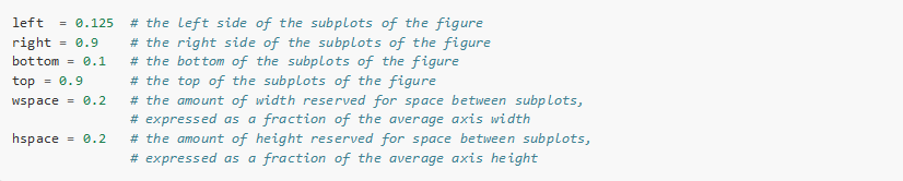
Taking the above figure as an example, considering that since the right side of the legend is not displayed, the right parameter of the subplots_adjust() function is adjusted to move slightly to the left, and the default value of the parameter right is changed from 0.9 to 0.8, then a complete legend can be obtained:
import numpy as np
import matplotlib.pyplot as plt

fig, ax = plt.subplots()

x1 = np.random.uniform(-10, 10, size=20)
x2 = np.random.uniform(-10, 10, size=20)
#print(x1)
#print(x2)
number = []
x11 = []
x12 = []
for i in range(20):
    number.append(i+1)
    x11.append(i+1)
    x12.append(i+1)
plt.figure(1)
# you can specify the marker size two ways directly:
plt.plot(number, x1, 'bo', markersize=20,label='a')  # blue circle with size 20
plt.plot(number, x2, 'ro', ms=10,label='b')  # ms is just an alias for markersize

lgnd=plt.legend(bbox_to_anchor=(1.05, 1), loc=2, borderaxespad=0,numpoints=1,fontsize=10)
lgnd.legendHandles[0]._legmarker.set_markersize(16)
lgnd.legendHandles[1]._legmarker.set_markersize(10)

fig.subplots_adjust(right=0.8)

plt.show()

fig.savefig('scatter1.png',dpi=600)
Compared with scatter.png, the effect of saving it as scatter 1. PNG is as follows:
As you can see, scatter1.png's legend is fully displayed. It is completed by moving to the left from the right position of the image and being included in the saved image as a whole.
Similarly, if the position of legend is at the bottom of the image and savefig() is incomplete, it is necessary to modify the parameter bottom of the function subplots_adjust() to move it upward, which is included in the box for the preservation of the intercepted image, that is, the bbox described below.
import numpy as np
import matplotlib.pyplot as plt
fig, ax = plt.subplots()
x1 = np.random.uniform(-10, 10, size=20)
x2 = np.random.uniform(-10, 10, size=20)
#print(x1)
#print(x2)
number = []
x11 = []
x12 = []
for i in range(20):
    number.append(i+1)
    x11.append(i+1)
    x12.append(i+1)
plt.figure(1)
# you can specify the marker size two ways directly:
plt.plot(number, x1, 'bo', markersize=20,label='a')  # blue circle with size 20
plt.plot(number, x2, 'ro', ms=10,label='b')  # ms is just an alias for markersize

lgnd=plt.legend(bbox_to_anchor=(0.4, -0.1), loc=2, borderaxespad=0,numpoints=1,fontsize=10)
lgnd.legendHandles[0]._legmarker.set_markersize(16)
lgnd.legendHandles[1]._legmarker.set_markersize(10)

plt.show()
fig.savefig('scatter#1.png',dpi=600)
Because the default bottom value in subplots_adjust() is 0.1, fig.subplots_adjust(bottom=0.2) is added to move the bottom up and change it to
import numpy as np
import matplotlib.pyplot as plt
fig, ax = plt.subplots()
x1 = np.random.uniform(-10, 10, size=20)
x2 = np.random.uniform(-10, 10, size=20)
#print(x1)
#print(x2)
number = []
x11 = []
x12 = []
for i in range(20):
    number.append(i+1)
    x11.append(i+1)
    x12.append(i+1)
plt.figure(1)
# you can specify the marker size two ways directly:
plt.plot(number, x1, 'bo', markersize=20,label='a')  # blue circle with size 20
plt.plot(number, x2, 'ro', ms=10,label='b')  # ms is just an alias for markersize

lgnd=plt.legend(bbox_to_anchor=(0.4, -0.1), loc=2, borderaxespad=0,numpoints=1,fontsize=10)
lgnd.legendHandles[0]._legmarker.set_markersize(16)
lgnd.legendHandles[1]._legmarker.set_markersize(10)

fig.subplots_adjust(bottom=0.2)

plt.show()
fig.savefig('scatter#1.png',dpi=600)
Effect comparison: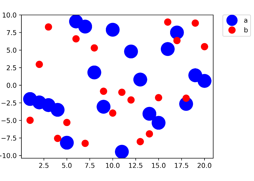
legend is the same in other places.
- Using the function savefig()
As mentioned in the last blog, three parameters in savefig() function, fname, dpi, format, can be used to save the vector graph. Now another parameter in this function, bbox_inches, is used to include the unsaved legends in the graph.
As you can see from the following figure, the bbox_inches function is to adjust the bbox of the graph, that is, bounding box.
As you can see, when bbox_inches is set to'tight', it calculates the tight boundary box bbox from the image and saves the image in the selected box.
The tighter bounding box here should be a rectangle that contains the image completely, but has a certain filling distance from the image. Personally, it is different from Minimum bounding box. The unit is also inch.
In this way, the legend will be included by bbox and then saved.
Complete code:
import numpy as np
import matplotlib.pyplot as plt
fig, ax = plt.subplots()
x1 = np.random.uniform(-10, 10, size=20)
x2 = np.random.uniform(-10, 10, size=20)
#print(x1)
#print(x2)
number = []
x11 = []
x12 = []
for i in range(20):
    number.append(i+1)
    x11.append(i+1)
    x12.append(i+1)
plt.figure(1)
# you can specify the marker size two ways directly:
plt.plot(number, x1, 'bo', markersize=20,label='a')  # blue circle with size 20
plt.plot(number, x2, 'ro', ms=10,label='b')  # ms is just an alias for markersize

lgnd=plt.legend(bbox_to_anchor=(1.05, 1), loc=2, borderaxespad=0,numpoints=1,fontsize=10)
lgnd.legendHandles[0]._legmarker.set_markersize(16)
lgnd.legendHandles[1]._legmarker.set_markersize(10)

#fig.subplots_adjust(right=0.8)

plt.show()

fig.savefig('G:/<Python Data Analysis and Application Learning Code/Chapter III/scatter2.png',dpi=600,bbox_inches='tight')
Save as scatter 2.png, the following is the comparison of scatter. png, scatter 1.png and scatter 2.png: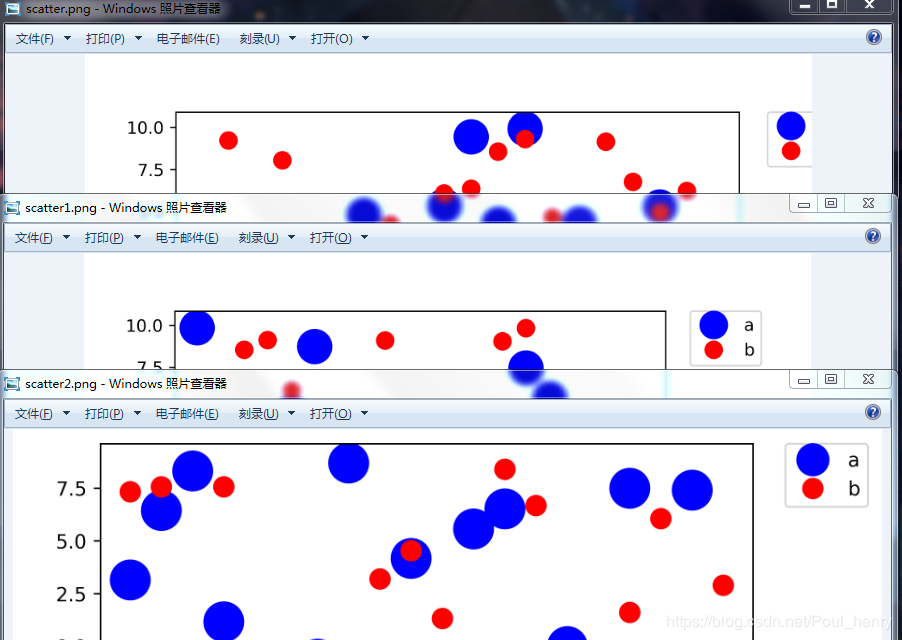
It can be seen that scatter 1.png, the idea of the first method, is to move the right edge of the image to the left and intercept the bbox unchanged, while scatter 2.png, the idea of the second method, is to expand the bbox of the intercepted image to the whole image directly and include it all.
Note: savefig() has two more parameters to explain
One of them is pad_inches. Its function is to adjust the filling distance between image and bbox when the current bbox_inches is'tight'. There is no need to set it here, just choose the default value.
Personally, if the pad_inches parameter is set to 0, i.e. pad_inches=0, the bbox saved by the captured image is the minimum bounding box.
The other is bbox_extra_artists, whose function is to include other elements when calculating the bbox of an image.
For example, if you add a text box to the left of the image and want the text box to be included in the bbox when saving the image, you can use the parameter bbox_extra_artists to include the text (in practice, even if bbox_extra_artists are not used, the saved image contains the text):
import numpy as np
import matplotlib.pyplot as plt
fig, ax = plt.subplots()
x1 = np.random.uniform(-10, 10, size=20)
x2 = np.random.uniform(-10, 10, size=20)
#print(x1)
#print(x2)
number = []
x11 = []
x12 = []
for i in range(20):
    number.append(i+1)
    x11.append(i+1)
    x12.append(i+1)
plt.figure(1)
# you can specify the marker size two ways directly:
plt.plot(number, x1, 'bo', markersize=20,label='a')  # blue circle with size 20
plt.plot(number, x2, 'ro', ms=10,label='b')  # ms is just an alias for markersize

lgnd=plt.legend(bbox_to_anchor=(1.05, 1), loc=2, borderaxespad=0,numpoints=1,fontsize=10)
lgnd.legendHandles[0]._legmarker.set_markersize(16)
lgnd.legendHandles[1]._legmarker.set_markersize(10)

text = ax.text(-0.3,1, "test", transform=ax.transAxes)

#fig.subplots_adjust(right=0.8)
plt.show()
fig.savefig('scatter3.png',dpi=600, bbox_extra_artists=(lgnd,text),bbox_inches='tight')
Display effect: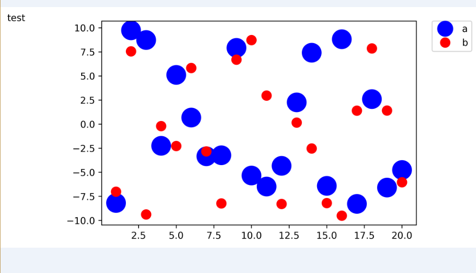
To prevent some elements from being included in bbox, consider using this parameter bbox_extra_artists